4C2 functional Materials

Functional materials course 4C2

Given that most of the electrical materials we interact with seem inert, why can we not treat them as such

Electrical materials can be treated as having loads of disordered dipoles. It is only when these dipoles are inside a electric field that they begin to align and result in a field.

A material that can be polarized like this is called a dielectric (not to be confused with this term also used for an insulator)

There are many types of dielectrics, but the ones where dipoles are always present but disordered are called polar dielectrics.

What are the types of dielectrics

The term paraelectric is used for dielectrics with a high response
This is often the case for ferroelectrics (with a permanent external dipole) above their transition temperature.

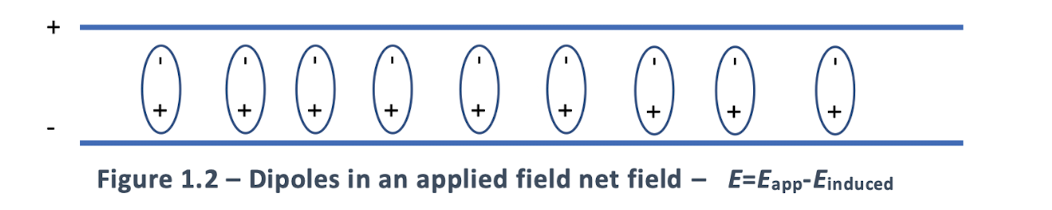
Dipoles in a field can be seen

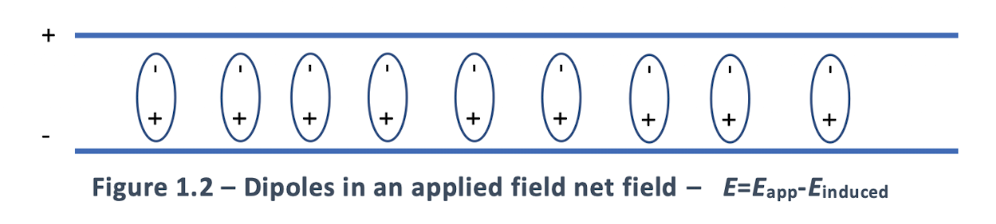
Effect of dipole field (in capacitors)

An induced dipole field opposes the applied field that induces it. This means this reduces the net electric field overall, meaning more charge requires in a lower voltage field in hte case of a capacitor.

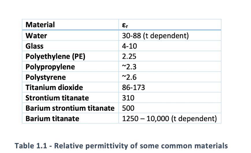
This is a big reason for trying to find materials with higher and higher dielectric constants.

Displacement field

From the dielectric, we have two contributors to electric fields.
There is the external field induced by charges on a capacitor, and also a polarisation field from dipoles being aligned which opposes this external field.

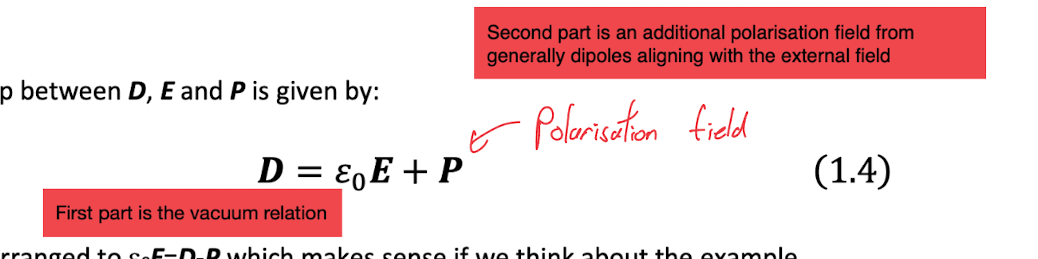
We can introduce a new quantity, called the displacement field to combine these two fields.

In a linear dielectric we can model the polarisation as P = ε₀χE , where χ is the electrical subsceptibility.

As we can write the displacement field as D = εᵣE, we can write the electrical subseptibility as (1 + χ ) = εᵣ

Remember that D is not a real separate field, but it just makes our problems easier

Origin of magnetic fields

Magnetics fields and electric fields are inherently one and the same as can be seen in maxwells equations.

We will see that magnetic fields originate from “moving” charges within atoms (electron).

We can take an analogy between electrostatic and magnetostatic fields, with the key exception that magnetic monopoles cannot exist

Magnetic field basics

As magnetic monopole cannot exist the base unit of magnetic fields is the magnetic dipole, analogue to an electric charge.

Magnetic fields can occur in two ways

• A flowing current in a wire, termed a Conduction current

• Intrinsic magnetic moments within materials and atoms, termed a Bound current

Units for magnetic fields

The conventional unit for magnetic fields is the magnetic flux or B-field, in units of tesla.

There is also the H-field or auxillary field, named auxillary as there is no SI unit, and is measured in A/m

We can understand this distinction with amperes law
∇ x B = μ₀j where J includes both the conduction currents AND bound currents, so this is analogous to the displacement field.

where as ∇ x H = jc where this only includes the conduction currents, more analogous to the E field.

Outside a material there is no difference, as there is no bound current, so they are just related with B = μ₀H

H fields inside magnets

Inside a magnet we will split the H field into an intrinsic H field that a magnetic acts on itself Hd and any external field from a flowing current as H₀
The total field H = Hd + H₀

Fields in free space and magnitude of magnetic fields

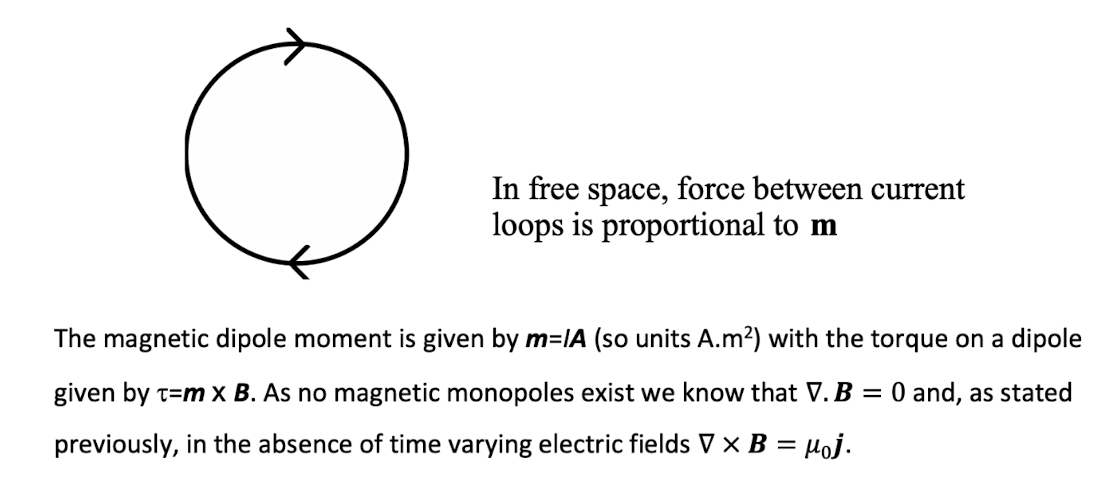
The simplest magnetic structure is a current loop, forming a magnetic dipole into and out of the page

Magnitude of magnetic fields

• Surface field of a strong perm magnet (eg neodynmium fridge magnet) : 0.3T

• Aligning all spins in a ferromagnet : 1.5T (this is the theoretical maximum for a perm magnet)

• Super conducting solenoids : 20T

• Explosive flux compression: 2500T

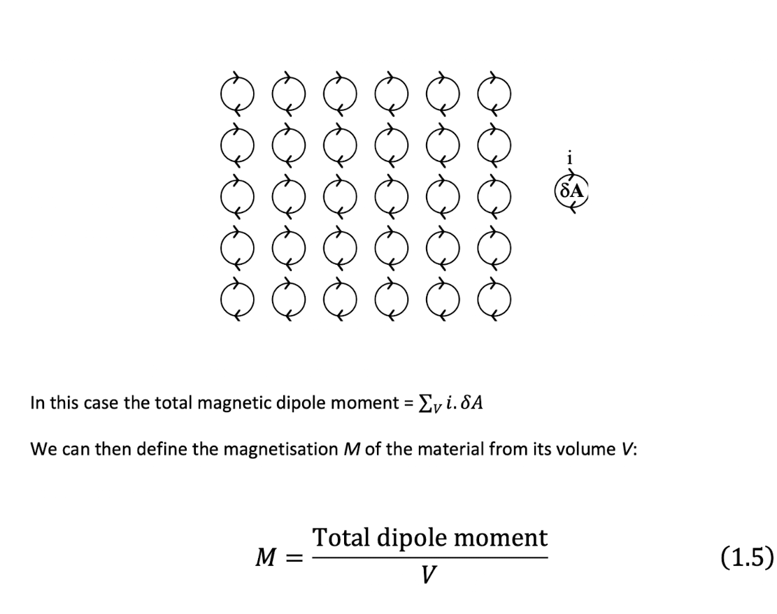
Magnetic fields in Materials (base equation)

Like in electric fields , we can represent magnetic fields in a material as a collection of spins, from this we can define a magnetiation field which is basically the density of magnetic dipole moments

We can link our parameters B, M and H together in a similar way to electric field, where we have a:

• Field due to magnetisation (from dipole alignment)

• Externally imposed field

So can write B = μ₀(M+H)

In real material, H isn’t just the external field, but also depends on M, as there is a demagnetisation field, but for long samples it effectively is just the external field.

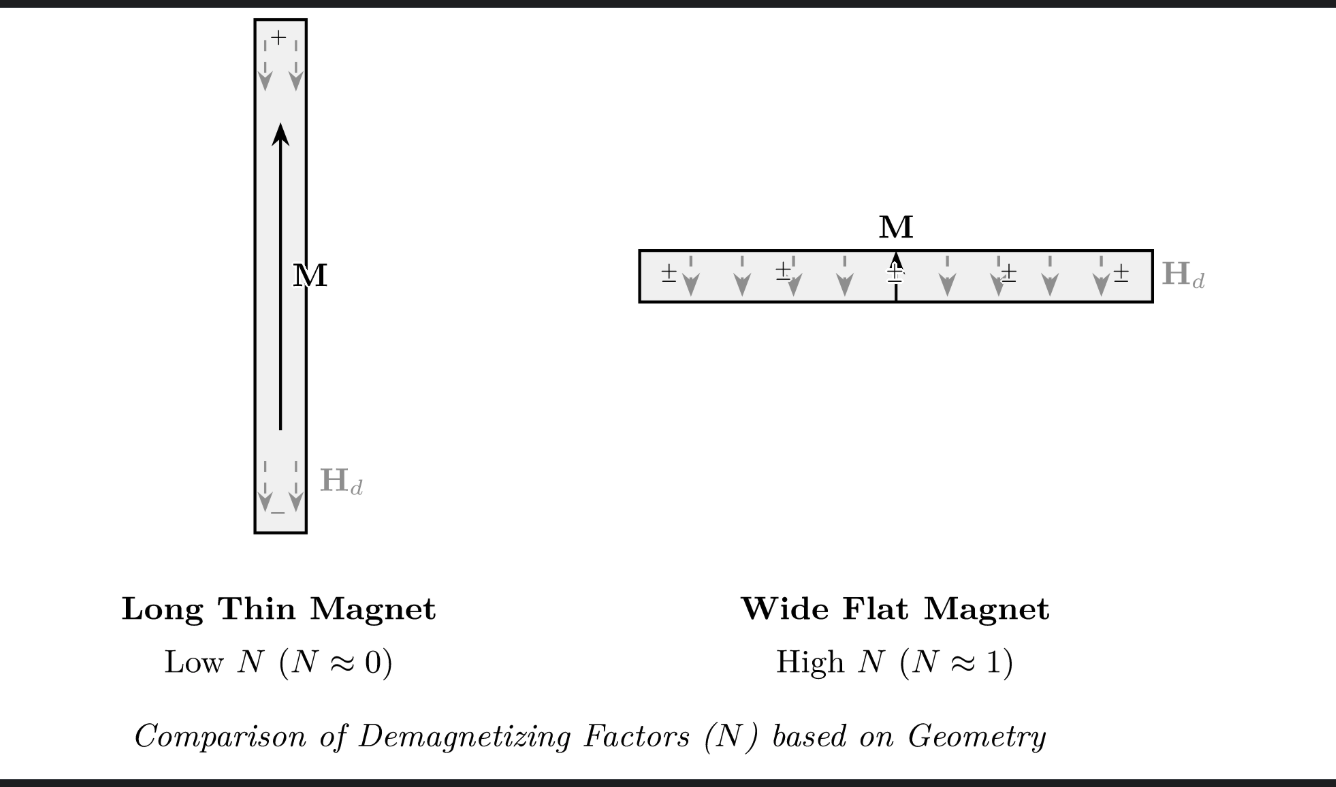
Explaining demagnetisation field

In a magnetic, especially permanant magnet the H field will not just be the external H field H₀ . Instead the magnet will induce a demagnetisation field on itself.

This makes the most sense if we imagine the magnetic field at a point. If we have a long thin magnet, our magnetic dipoles will add up linearly and won’t oppose each other. But if we have a wide flat magnet, the adjacent magnetic bits will result in an opposing field, this is our demagnetisation field, so there is a significant different from just the magnetisation field.

This varies with different shapes

Material parameters

In general the magnetising field depends on the external field, because the strong the external field is, the better it works at aligning the magnetic dipoles within a material resulting in a differing magnetising field. (Our atomic dipole moments are generally randomly aligned (in a non ferromagentic material))

For a non ferromagnetic material, this relationship is typically linear
M = χH

χ is magnetic suscpetibility often written as χₘ to distinguish it from electrical susceptibility. This is a measure of how easy it is to align atomic dipole moments.

Varying types of magnetic material

There are three types of magnetic material

• Diamagnetic materials have χ < 0 so appear to expel magentic field

• Paramagnetic materials have χ > 0 so concentrate magnetic flux lines.
  

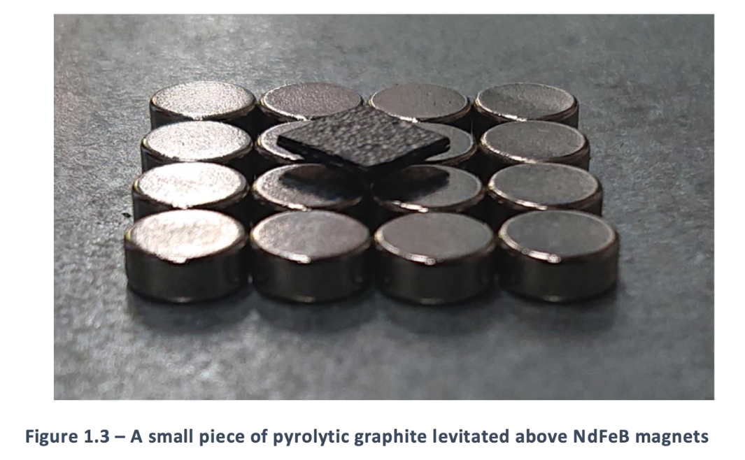
Most materials are very weakly para or diamagnetic so we don’t really notice some, clear exceptions are bismuth and pyrolytic graphite which are strongly diamagnetic and can levitate!!

Table -χₘ/10⁻⁵
Copper: 1
Silver : 2.6
DIamond: 2.1
Water: 0.91
Pyrolytic graphite: 40
Bismuth: 16.6
Hydrogen gas: 0.00021

Mechanism of action:
For diamagnetism, this occurs because the external magnetic field affects the already paired spin up and spin down electrons differently. Without a field these electrons cancel out so there is no intrinsic magnetic moment, but with an external field, the interaction resutls in an oppositely oriented magnetic dipole

For paramagnetism, this occurs due to the alignment of unpaired electrons with the field, this dominates over the diamagnetic effect of the paired electrons

Thermal oscillations result in random alignmnet without an external field

Introduction to Ferromagnetism

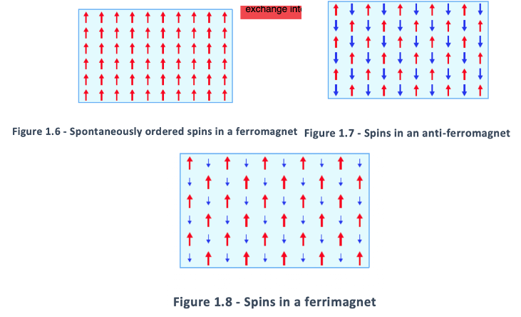
Practical magnetic materials are ferro magnetics where the magnetic dipoles spontaneously align due to a quantum mechanical exchange interaction.

There are three types of ferromagnets:

• Ferromagnets where the spins align with each other

• Anti ferro magnets where the spins align to oppose each other resulting in no resulting magentisation

• Ferrimagnets, which are anti ferromagnets but the two dipoles have differeing strengths resulting in an overall magnetisation
  

How magnetised can a material get

There is a limit to magnetism, which can be estimated given that fields in ferromagnetic materials are generated by aligned spins.

Each of these spins have a quantised magnetic dipole of 1Bohr , μB = eh/4πm = 9.27 × 10⁻²⁴ Am²

Magnetic moment is therefore a quantised quantity in terms of bohr.

Iron has on average 2.2 unpaired spins per atom (more than cobalt at 1.72 and nickel at 0.6) given the lattice spacing of iron we can work out the maximum possible magnetisation which is 1.7T

As such fields generated by permanent magnets remain below 2T

Spontaneous magnetisation in ferromagnets

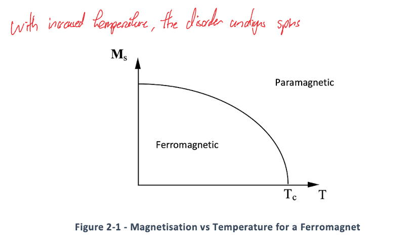
Most metals are paramagnetic, because of thermal oscillations resulting in non aligned spins.

However, with ferro magnets a quantum exchange interaction results in neighbouring spins aligning with each other. There are only three ferromagnetic materials in nature, iron (bcc), ni(fcc), co(hcp)

Here we can see how with increasing temperature, thermal oscillations can overcome this quantum exchange interaction and result in the disordering of the spins.

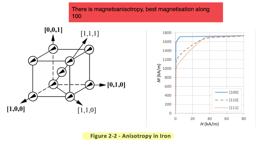
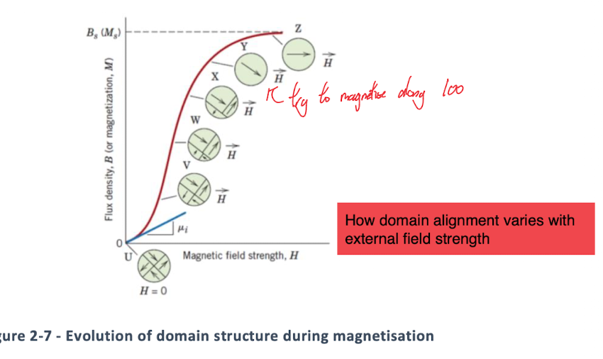
Magneto anisotropy

With BCC iron the magnetic moments align most easily with the principle crystallography directions <100>

However with a stronger H field, the magnetisation converges to the maximum magnetisation where all the spins are aligned with the auxillary field,

We can see how the propensity for magnetisation varies with direction.

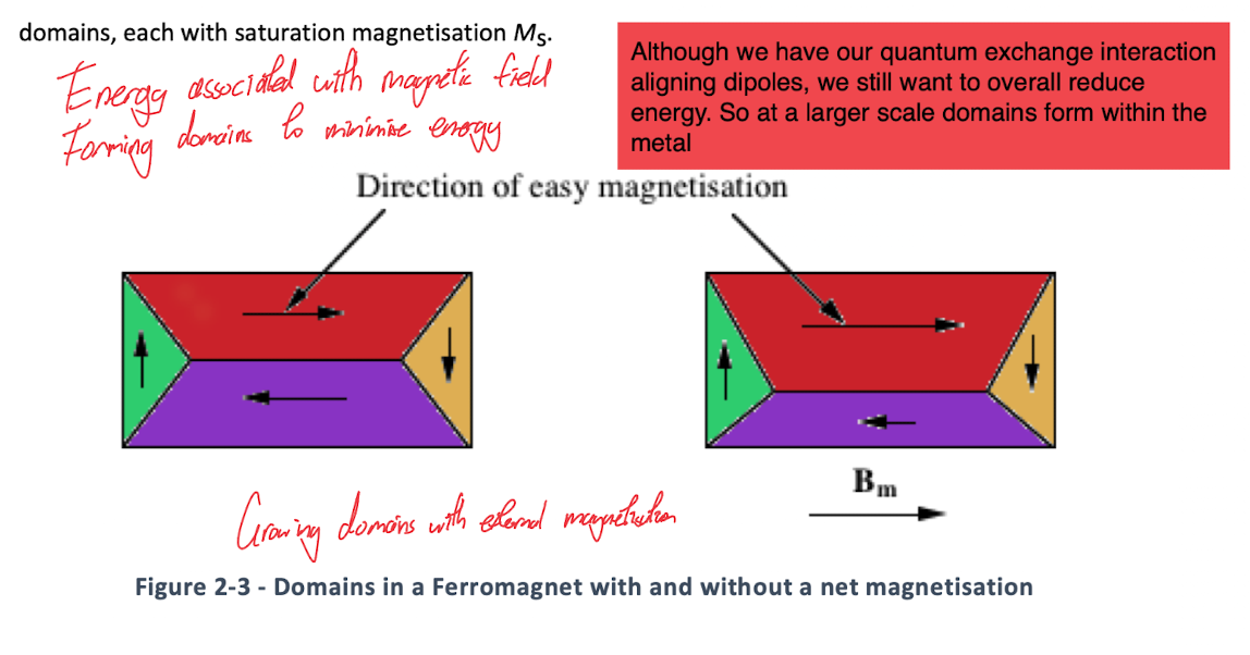
Ferro magnetic domains

Although we have the quantum exchange interaction aligning dipoles, this is still thermodynamically unstable, and we would want to minimise the energy from the magnetic field. As such the aligned dipoles form into regions known as domains, which are randomly oriented to result in no net magnetisation.

With a growing magnetic field, the domains which are already aligned with the external auxillary field grow in size resulting in increasing magnetisation.

we have two types of magnetic materials, soft and hard based on how easily these domains move. The domain walls can be pinned in position resulting in permanent magnets. Pinning is a source of hysteresis resulting in energy loss which increases with frequency.

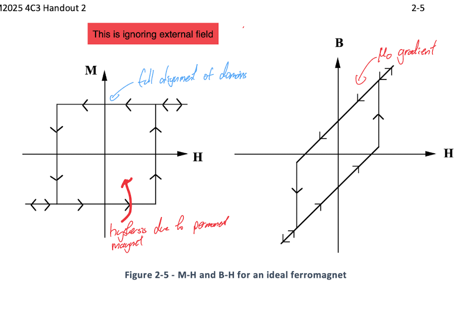
B-H curve in permanent magnets (ideal)

Here measuring the B-H curve for a long rod (to minimise any demagnetisation effects) for ferro magnetic materials

With an ideal ferromagnet we would have instantaneous fully alignment of the the magnetic domains resulting in square magnetisation curve which caps out at the saturation value. Including the H field on top of this we get our ideal B-H curve as shown.

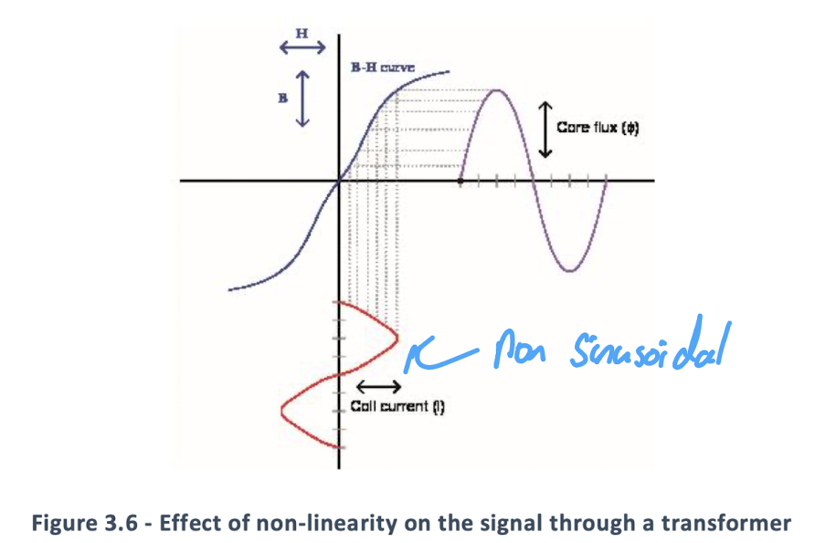
B-H curve in ferromagnetics (real)

With real magnetic materials, we have a more complex non linear curve. Here we can see we are conflating B and M together because the magnetising field is much much bigger than the auxillary field that induces it.

At low field strengths, the magnetising field lags behind the auxillary field due to domain boundary pinning
At higher strengths we get a roughly linear increase in magnetisation as the domain best aligned with the magnetic field grows
At even higher fields we have a slower increase in magnetistaion as the domain rotates to align with the field, until we hit saturation where the domain is fully aligned

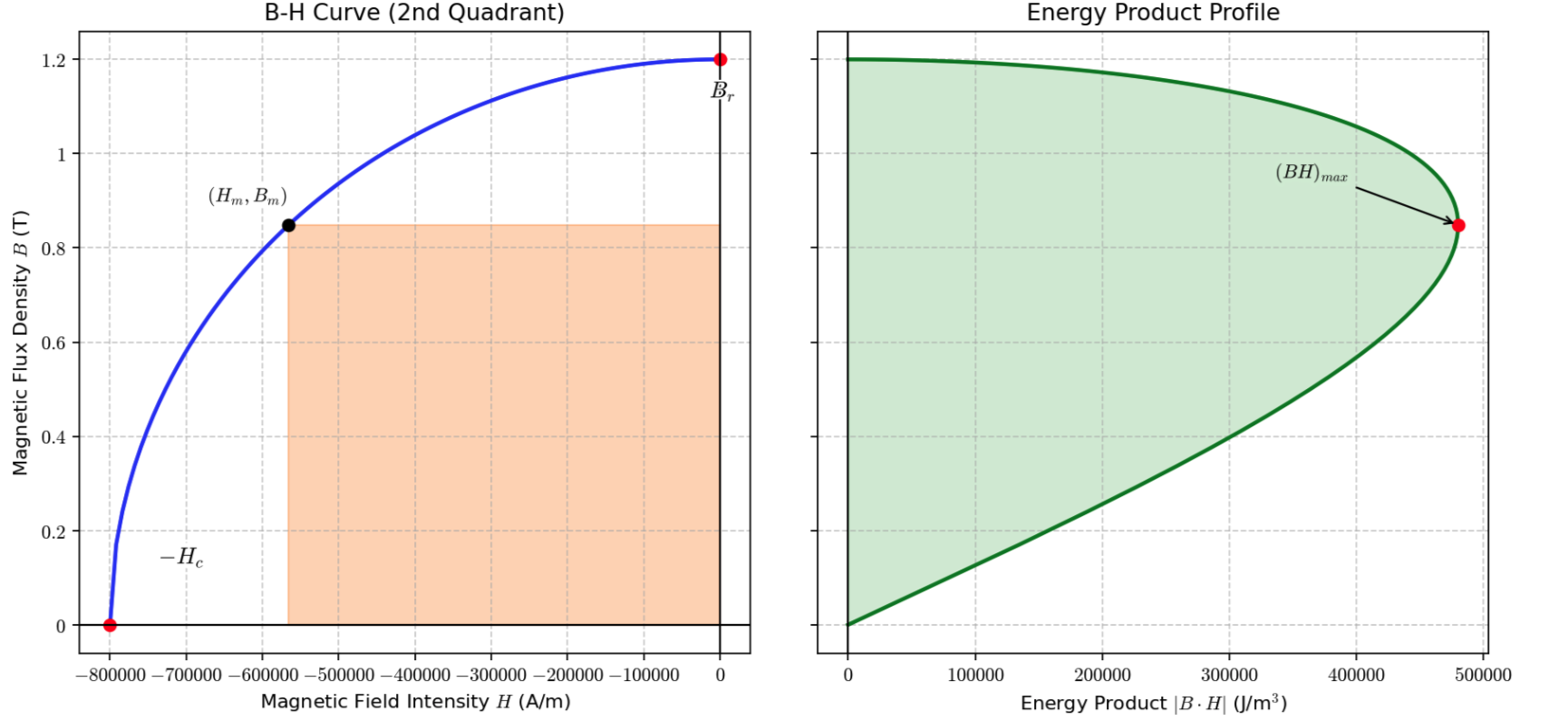
BH max the operating point for magnets

Basically the best operating point for our magnet is maximising the product of BH. This is because this maximises the magnetic energy generated by the magnet. When using a magnet we want to drive the largest flux through an airgap with as little magnetic material as possible, maximising the magnetic energy achieves this.

The operating point is on the second quadrant because this means the demagnitising field is working against the magnet and it means we have done work into the magnet.

For a linear magnet material as B = μH with a line intersecting the y axis at M_sat, and the fact that our stored magnetic energy = ½BH, this means our maximum magnetic product is at H = M_sat / 2

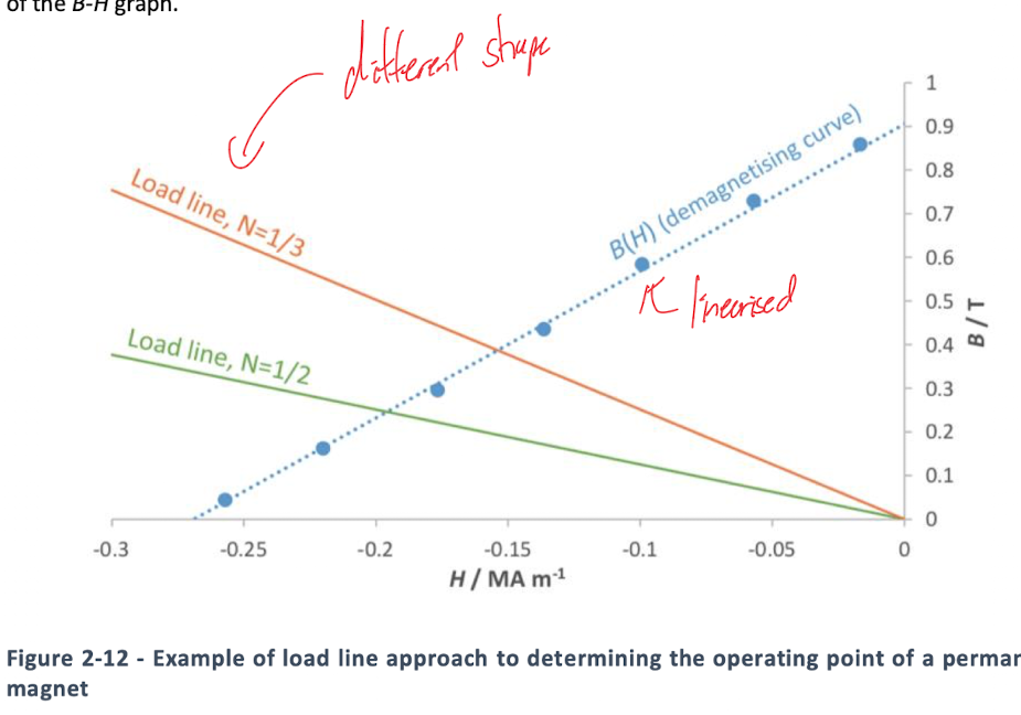
Demagnetising field and geometry changing the operating point

As mentioned earlier varying shapes of magnets will result in different demagnetising fields as the magnet, we can tailor the shape of the magnet to change the demagnetising field, this field generates the auxillary field that sets our operating point or our load line.

A very long magnet will have almost no demagnetising field, so there is very limited stored magnetic energy, while a very flat magnet will have such a high demagnetising field that we’re almost completely cancelling our our magnetising field so there is no magnetic flux.

For an application such as a fridge magnet where there is no external H field, to maximise the stored magnetic energy to maximise the airgap flux, we want the shape of the magnet to have a “demagnetising factor” of ½. This means the demagnetisation field is a half of the magnetising field, reaching our maximum energy operating point.

However, for say a motor, where there is an additional H field beyond the demagnetising field, we would want this magnet to have a lower demagentising field, so the combined H field would result in this maximum energy operating point.

N values for varying shapes
1 Flat plate
0 Infinite thin rod (field parallel to axis)
½ Infinite cylinder (field perpindicular to axis)
1/3 sphere
~½ squat disc (h ≈ r)

This ½ factor for a squat disc is why most fridge magnets are this shape

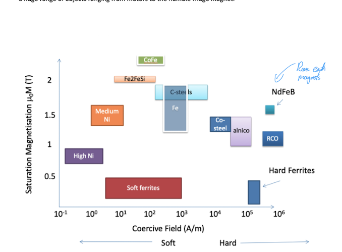
Ashby plot of magnetic materials

Various magnetic materials on a plot, a high coercivity means it is hard to demagnetise resulting in a “hard magnet”

high saturation means we can have a stronger field (magnetisation) before saturation

Examples of magnetic materials (irons and steels)

Mostly used for cheap soft ferromagnets, pretty terrible for permanent magnets due to poor coercitivity so it is really easy to demagnetise and bad saturation too.

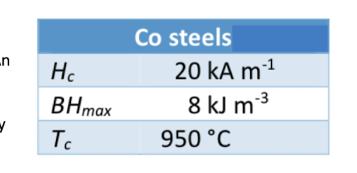
Cobalts can be added to greatly improve the coersivity and saturation field, and has a very high curie temperature. Hard magnetic steels are almost always quenched to produce a highly stressed martensitic structure that helps pin the domain boundaries.

Examples of magnetic materials (ALNICO)

This is a family of materials that superseeded martensitic steel permenant magnets
Iron based material with a mixture of Fe, Ni, Al and significant cobalt.

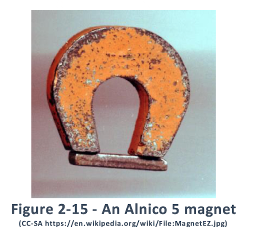
Unlike the steel magnets they are hard and brittle, so are generally made using casting or powder methods, and have fairly constant properties up to 400 degrees c>

They can be separated into isotropic alnicos and anisotropic alnico which is introduced via texturing (grain orientation) or processing in a magnetic field.

We can see an alnico magnet above, the horseshoe shape is to minimise the demagnetisation field with a more rod like shape. A plate is put there to prevent magnetisation forming a magnetic loop. This is no longer necessary with modern rare earth magnetics which have a much higher coersivity

Hc = 40-160kA m⁻¹
BH = 10-74 kJm⁻³
Tc = 810-900C
Tmax = 450-550

Example of hard magnetic materials Hard ferrites

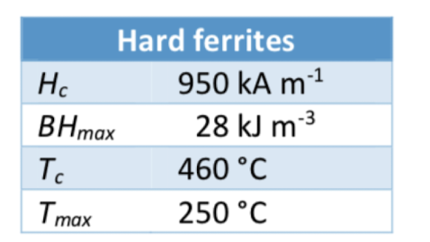
Ferrites refer to a iron oxide based magnetic material. Hard ferrites typically have a magneto plumbite structure with the formula MFe₁₂O₁₉ where M is barium, strontium or lead. Often called hexaferrites due to the structure.

The Fe³⁺ ions responsible for the magnetism are distributed among three typers of lattice site with varying orientations, with the total unit cell having a magnetisation of 40 bohr.

Saturation magnetisation is quite poor, but has really good coersivity due to crystalanisotropy and small particle particle size basically each particle is it’s own domain so there’s no domain growth mechanism only the domain rotation. The ferrite also tends to form flat plates (which the field will be in plane to minimise demagnisation) so when stacked together there is generally some magnetic alignment.

Very low cost, and high coersivity so still often used.

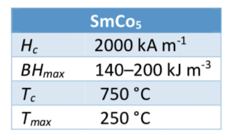
Example of hard magnetic materials SmCO

SmCo intermetallic, hard and brittle, very expensive but very good coersivity and saturation. Powder route with small domain sized particles sintered together. Relatively high maximum operating temperature.

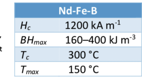
Example of hard magnetic materials NdFeB

Very common rare earth magnet, very good coersivity and saturation. Powder route is typically taken, and corrosion is an issue so it’s often chromium plated. Kind of low curie temperature.

Loads of geometric flexibility, even quite flat magnets due to the high coercivity

Requirements for soft magnetic materials (eddy and hysterisis losses)

For soft magnetic materials we want as low of a coersivity as possible to reduce energy loses due to hysterisis, for very high frequencies eddy cuerrents also become an issue and we’d want a high resistance or insulating material or use laminations to limit the size of current loops. (Trains in De run at 50/3 Hz to minimise these losses)

The losses due to eddy currents in thin sheet are given by P = B²t²f²/ ρ where ρ is the resitivity, B is the peak flux and t is the thickness, this shows why eddy losses become a big issue at higher frequencies, as well as why very thin laminations are so effective at reducing eddy losses

We still want a high saturation field as possible

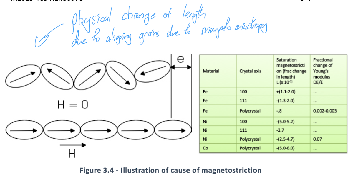
Magnetostriction

From the anisotropy of magnetic materials, we can cause a change in shape of material when applying a magnetic field, as the crystal structure aligns to align with the external field, this can be a significant cause of losses and causes the buzzing sound from transformers.

Soft magnetic materials: Shape of B-H curve

We want different B-H curves depending on the application of our soft magnetic material

A flat curve for low loss - good for a transformer
Round curve with high μ this is good for compact electronics
Square curve for switching like in an HDD.

In addition if we want a transmit a signal, ie for an inductor we want a linear response.

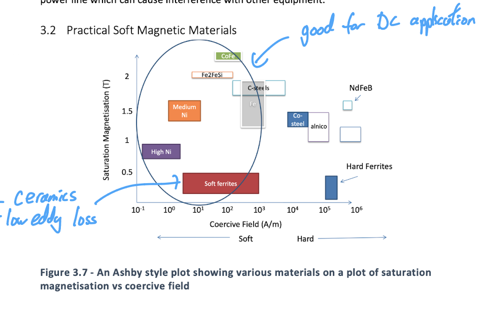
Ashby plot for soft magnetic materials.

We want low coercivity in all cases, but for high frequency ferrites become attractive despite their low saturation because they are non conductive ceramics, minimising eddy losses

Soft magnetic materials : irons and steels

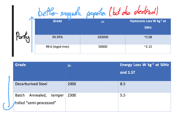
Pure iron can have a very high relative permability, and low coercivity if anneals and coarse grained.

More typical irons and low carbon steels have significantly worse propoerties but much cheaper, so are widely used for low frequency applications where the coercivity does not matter such as pole pieces for electromagnets

For low cost AC applications, these typical irons can still be acceptable, with laminated sheets (insulated) used to minimise eddy losses, as eddy losses scale with t². Often insulated with an iron oxide film.

Soft magnetic materials : Silicon steels.