sampling, contrast, pixel ops

Concise computer vision: 1.1, 2.1

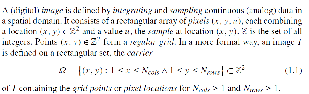
Image in spatial domain

Adjacent pixels

we may assume that pixel locations are adjacent iff they are different and their tiny shaded squares share an edge. Alternatively, we can also assume that they are adjacent iff they are different and their tiny shaded squares share at least one point (i.e. an edge or a corner).

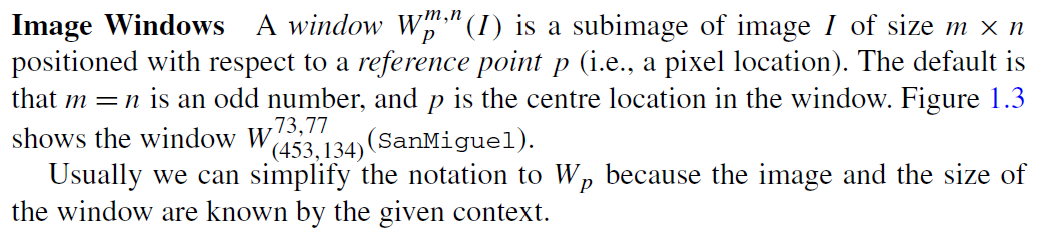
Image Windows

Binary image

A binary image has only two values at its pixels, traditionally denoted by 0 = white and 1 = black, meaning black objects on a white background.

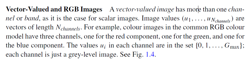
Vector-Valued and RGB Images

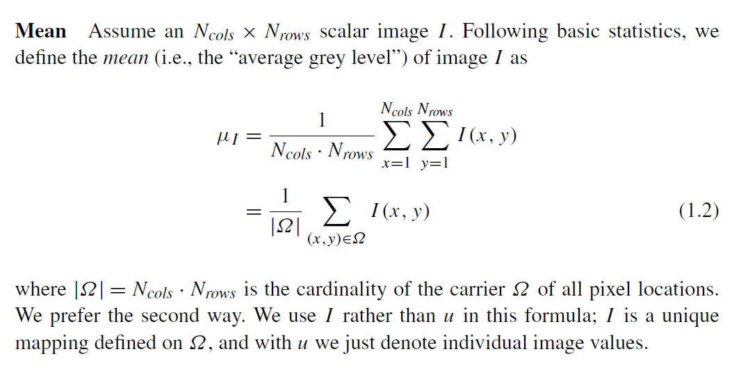
Mean (or avg grey level) of an image

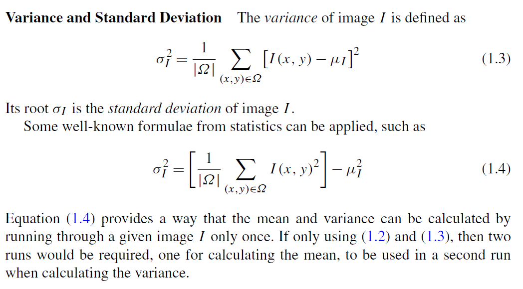
Variance and standard deviation of an image

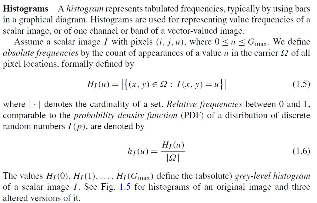
Histograms

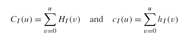
Absolute and relative cumulative frequencies

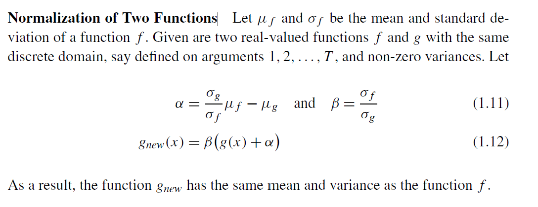
Normalization of Two Functions

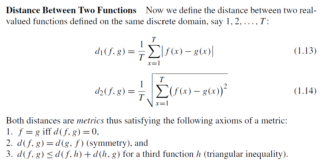
Distance between two functions

What’s an edge?

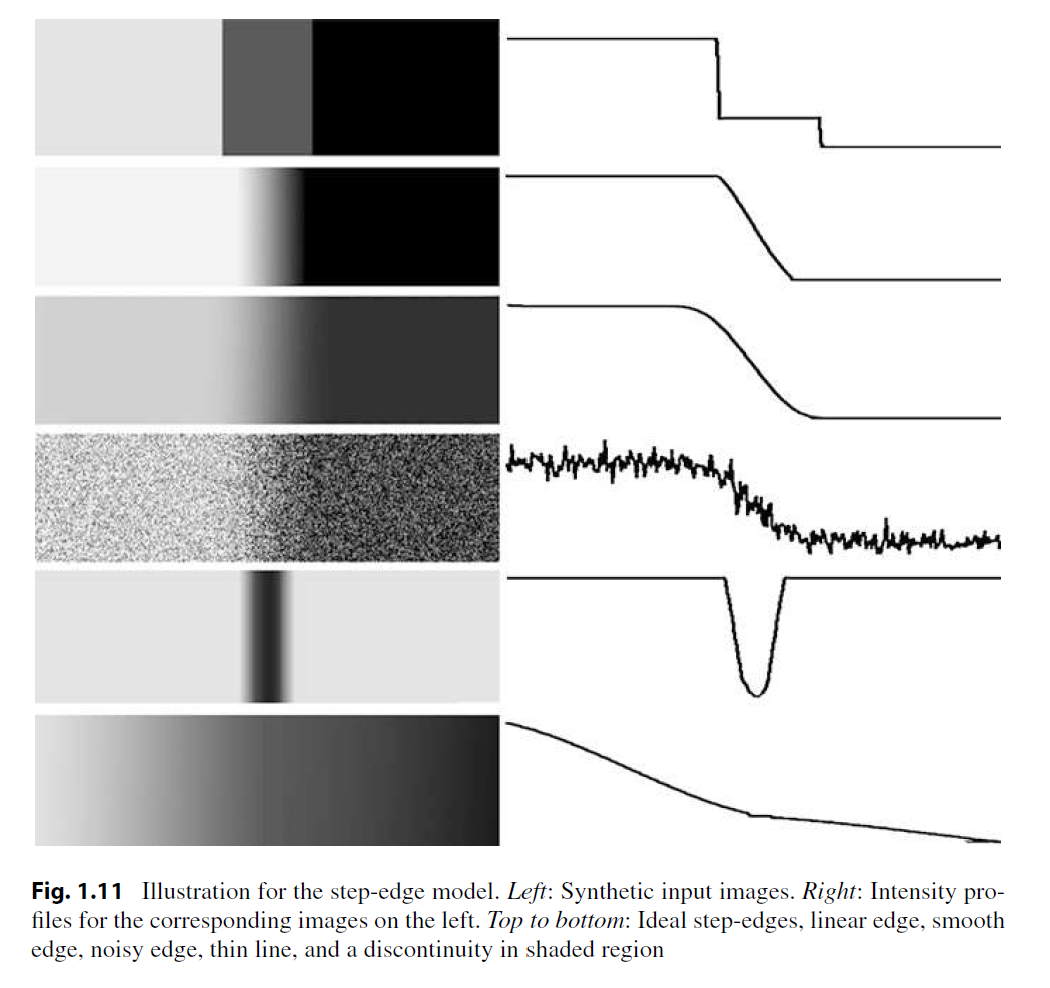
Figure 1.11 illustrates a possible diversity of edges in images by sketches of 1D cuts through the intensity profile of an image, following the stepedge model. The step-edge model assumes that edges are defined by changes in local derivatives; the phase-congruency model is an alternative choice.

After having noise removal performed, let us assume that image values represent samples of a continuous function I (x, y) defined on the Euclidean plane R2, which allows partial derivatives of first and second order with respect to x and y.

Detecting Step-Edges by First- or Second-Order Derivatives

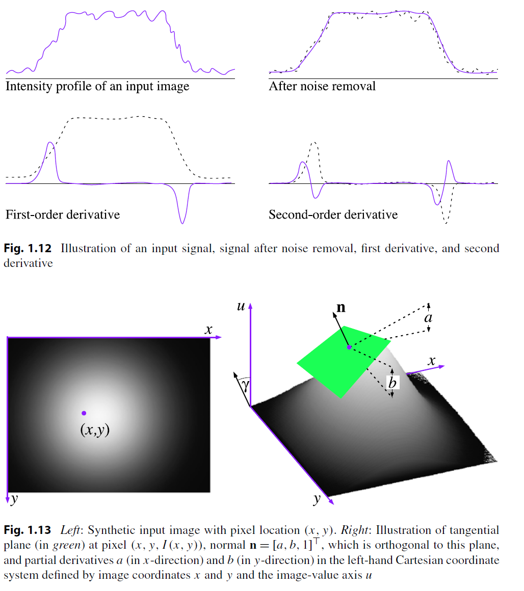
Figure 1.12 illustrates a noisy smooth edge, which is first mapped into a noise-free smooth edge (of course, that is our optimistic assumption). The first derivative maps intervals where the function is nearly constant onto values close to 0 and represents then an increase or decrease in slope. The second derivative just repeats the same taking the first derivative as its input. Note that “middle” of the smooth edge is at the position of a local maximum or local minimum of the first derivative and also at the position where the second derivative changes its sign; this is called a zero-crossing.

Def of noise

An unwanted data is called noise. These are three examples of noise in this sense of “unwanted data”. In the first case we may aim at transforming the images such that the resulting images are “as taken at uniform illumination”. In the second case we could try to do some sharpening for removing the blur. In the third case we may aim at removing the noise.

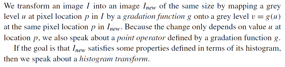
Gradation functions

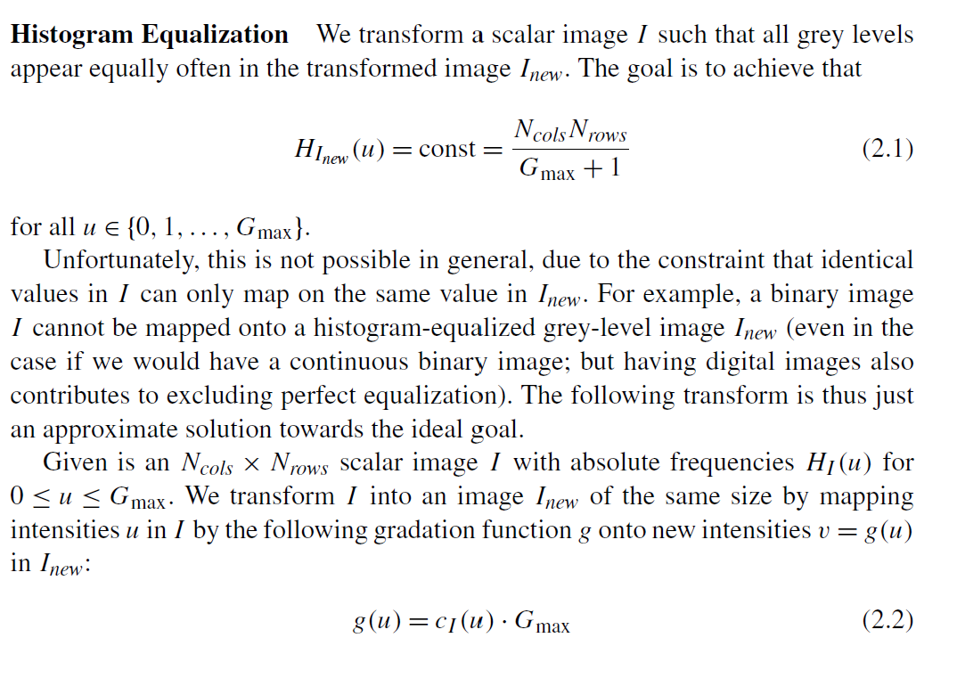
Histogram equalization

where cI is the relative cumulative frequency function.

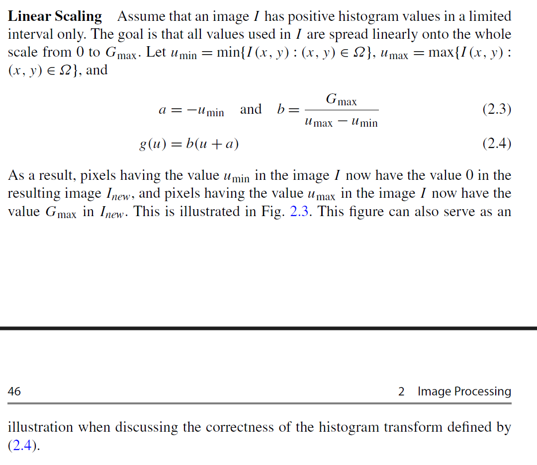
Linear scaling

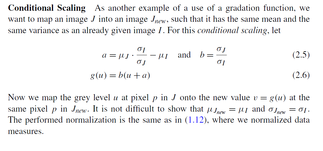
Conditional scaling

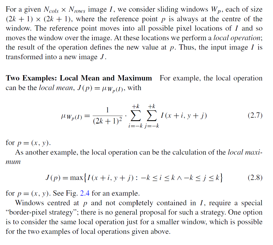
Local Mean and Max

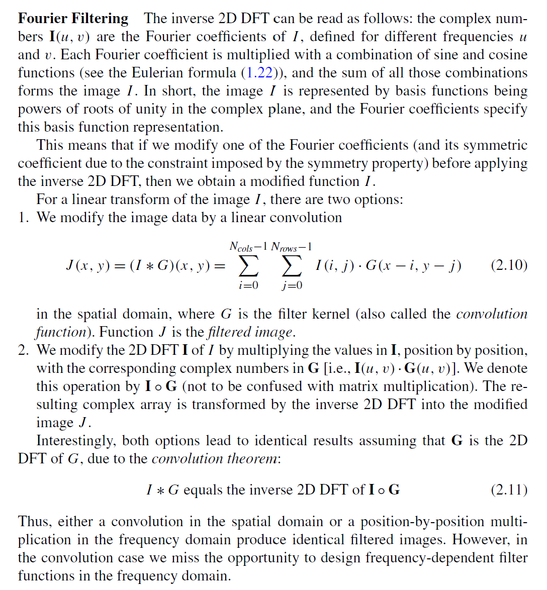
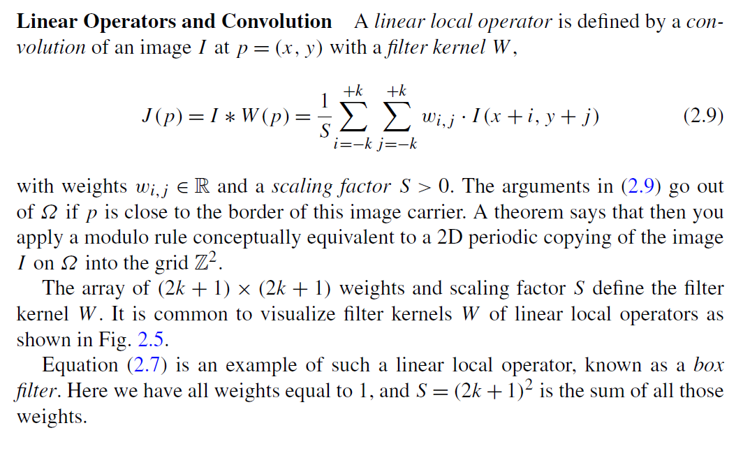
Linear Operators and Convolution

Fourier Filtering