Linear Models

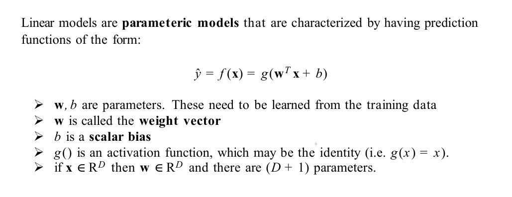
Linear Models

Linear models are parameteric models that are characterized by having prediction functions.

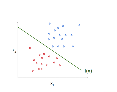
Classification with Linear Models

When using a linear model for classification, we are interested in which side of the line f (x) = c the target appears on.

Regression with Linear Models

When using a linear model for regression, we simply output the value of y = w^Tx + b.

Why linear models?

• Even if there is no linear relationship (or decision boundary), often possible to project data to a space in which relationship is linear.

• If you have very little data, you need to make strong assumptions to fit a model. Low variance.

• Occam’s razor (principle of parsimony). Simpler models that explain the data are better than more complicated ones.

• Possible to build much more complex models using linear models as a building block. This is the basis of neural networks and deep learning.

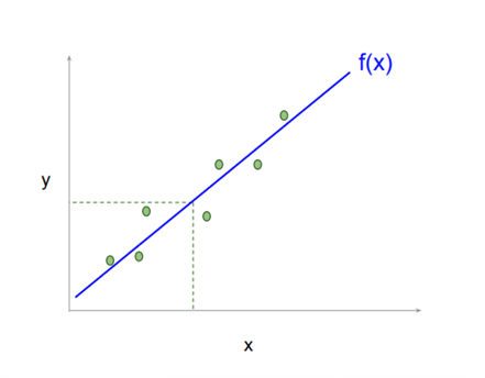
Linear Regression (Ordinary Least Squares)

In linear regression, we would like to find parameters {w, b} such that the resulting line f (x) fits the training data well.

Loss (Cost) Function

A loss function measures how wrong a model’s prediction is for a single data point.

Normal Equations

The Normal Equations give a direct solution for finding the best-fit parameters in Linear Regression by minimizing Mean Squared Error.

Gradient Descent

An iterative optimization algorithm used to minimize a loss (cost) function by repeatedly moving in the direction of steepest decrease.

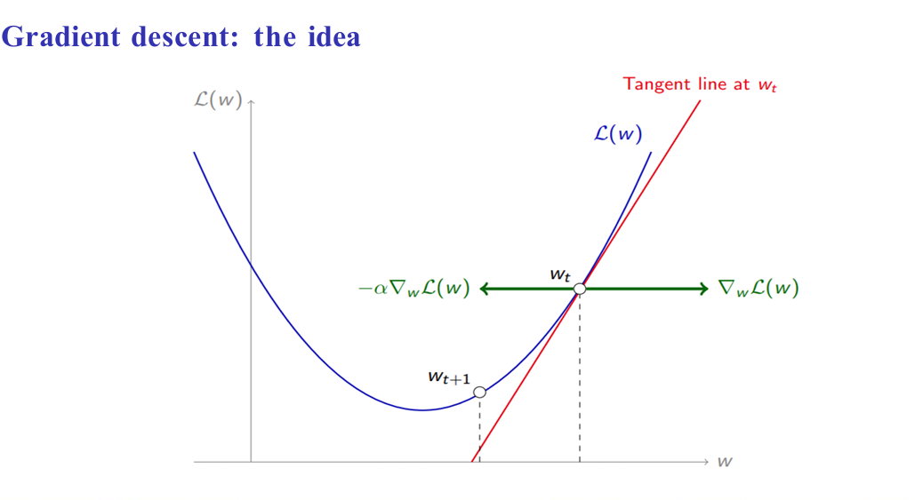
Gradient Descent: The Algorithm

1. Start with a random guess for the initial parameters θ₀

2. While not converged:

   • Set θ_t+1 = θ_t − α_t∇_θL(θ_t)

Gradient Descent: When to Decide Convergence

The value of α_t is called the learning rate. Decide convergence when:

• The change in θ is small |θ_t+1 − θ_t| < T

• Maximum number of iterations are reached.

• Loss stops improving.

Properties of Gradient Descent

The learning rate α_t :

• Gradient descent will converge on convex functions as long as the learning rate αt keeps getting smaller over time.

• Gradient descent may be very slow if α_t is too small.

• Gradient descent may diverge if α_t is too large.

Gradient descent requires a full pass over the dataset each time it updates the parameters (weights and biases). Slow for large datasets.

Stochastic Gradient Descent (SGD)

Instead of computing the gradient of the loss for the full dataset, estimate it using a single randomly chosen example and then take step in that direction.

Properties of SGD

• Usually much faster than batch gradient descent, since we update the weights every iteration instead of every epoch.

• Can operate on large datasets, since we only need to process a single example at a time.

• Important to shuffle training data to ensure the gradient estimates are unbiased (i.i.d.)

Cons of SGD

• Gradient updates are noisy, since it is only an estimate of the full gradient.

• Convergence may be slower as you near the optimum solution.

Assumptions of Linear Regression

• Linear relationship between variates and covariate

• All other variation can be modelled as zero mean Gaussian noise

If these assumptions are violated, then linear regression may be a bad model.

Implications of Linear Regression

• Linear regression is sensitive to extreme outliers.

• Linear regression may not be appropriate when the noise is not Gaussian.

• Linear regression may not give good results if the relationship between the variates and covariates is not approximately linear.

Is it possible to use our linear regression model to do classification?

Sure, but it probably won’t work very well.

• The relationship between the variates and covariates is not directly linear

• We would like our outputs to be binary variables in {0, 1} (or probabilities in [0 . . . 1]), but linear regression produces arbitrary real numbers. We would need to do some post processing to map the values to the desired range.

• Assumption of Gaussian noise is not true for binary outputs. So square error is inappropriate.

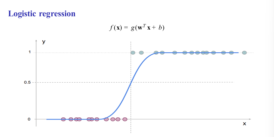
Logistic Regression

A supervised learning algorithm used for binary classification problems, where the output is either 0 or 1. It works by applying a linear model to the input features and then passing the result through the sigmoid function, which converts the output into a probability between 0 and 1. The model predicts class 1 if the probability is greater than or equal to 0.5, otherwise it predicts class 0.

Components needed to specify the logistic regression algorithm?

1. An activation function (transfer function): the logistic sigmoid

2. An appropriate loss function (cross-entropy) derived using maximum likelihood

Logistic Regression: Loss Functions

To fit the parameters we would also like to use a more appropriate loss function than square loss:

• Probability Distribution

• Binary Cross Entropy Loss

Gradient Descent for Logistic Regression

Perform gradient descent (or SGD) using the usual update rule to find good parameters.

Linear regression: Fitting Polynomials

Possible to use linear regression for more than just fitting lines! Only needs for function to be linear in the parameters

! Feature Mapping Function φ(x)

Feature Engineering

Good features are often the key to good generalization performance.

• Low dimensional: less likely for data to be linearly separable

• High dimensional: possibly more prone to overfitting

Process of designing such functions by hand is called feature engineering, but it is notoriously difficult.

! Feature Learning

Learn features from the data directly.

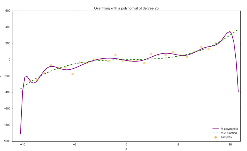
Overfitting

If the model has too many degrees of freedom, you can end up fitting not only the patterns of interest, but also the noise.

• This leads to poor generalization: model fits the training data well but does poor on unseen data

• Can happen when the model has too many parameters (and too little data to train on).

Curse of Dimensionality

• Estimation: more parameters to estimate (risk of overfitting).

• Sampling: exponential increase in volume of space.

• Optimization: slower, larger space to search.

• Distances: everything is far away.

• Harder to model data distribution P(x₁, x₂, . . . , x_D )

• Exponentially harder to compute integrals.

• Geometric intuitions break down.

• Difficult to visualize

Blessings of Dimensionality

Linear separability: easier to separate things in high-D using hyperplanes

! Dimensionality

! Multiple Regression

Multi-Class Classification

Logistic regression is limited to binary outputs {0, 1}. Often, if we want to do multi-class classification: Output is one of K classes {1, 2, . . . , K}

How do we model Multi-Class Classification?

Two approaches:

1. One-vs-rest (OVR): aka one-vs-all

2. Softmax regression

! One-vs-Rest (OVR)

Idea: train K separate binary classifiers.

! Softmax regression

Direct extension of logistic regression to the multi-class case.

! Loss function for Softmax regression

categorical cross entropy

Regularisation