Population ecology

λ

N_t+1/N_t, 1+b-d

Finite per capita rate of population growth for discrete-time population growth model

finite rate of population change over a given time interval (often a year)

discrete-time population growth model

N_t+1 = N_t(1+b-d)

geometric population growth model

N(t) = N(0) λ^t

Cumulative finite rate of increase

100((Nt+5/Nt )-1)

If Nt + 5 = 128 and Nt is 100, then (128/100)-1 = 28%

Thus, the population has grown by 28% over 5 year

Time to reach a given population size

log(Nt) = log(N0)+t(logλ)

Stable Age Distribution

When a population is growing exponentially: the proportion of individuals in each age (or stage) class becomes stable and remains constant; each age class grows at the same exponential rate of increase

Assumptions of the Geometric Growth Model

1. Individuals in the population breed during a discrete

time period

2. Nothing changes from year to year except population abundance

3. Assumes the same birth and death rates for each

individual

4. Treats males and females the same

R0

the net reproductive rate per generation

Where species are annual breeders that live one year

R0 = λ

Generation growth

Nt = N0R0t, where t = a number of generations

What's not different between R 0 and λ

Populations grow when R0 or λ > 1

Populations decline when R0 or λ <1

Populations are at equilibrium when R0 or λ =1

Geometric Growth Model use

Appropriate when a population breeds during discrete times, where R0 = λ (annual breeders)

Exponential growth model

The rate of population increases under ideal conditions

exponential growth model equation

dN/dt = rN

○ dN/dt is the population growth rate (continuous breeders)

○ N is the population size

○ r is the instantaneous per capita rate of population growth

Exponential growth Nt equation

Nt = N0e^rt

r>0

population is growing exponentially

r<0

population is declining

r=0

population stable

R0 & r

R 0 & r are similar; give similarly shaped growth curves

○ R 0 reflects a generational growth rate

○ r denotes an instantaneous rate

○ Rough approximation: r ≈ ln R0 /T

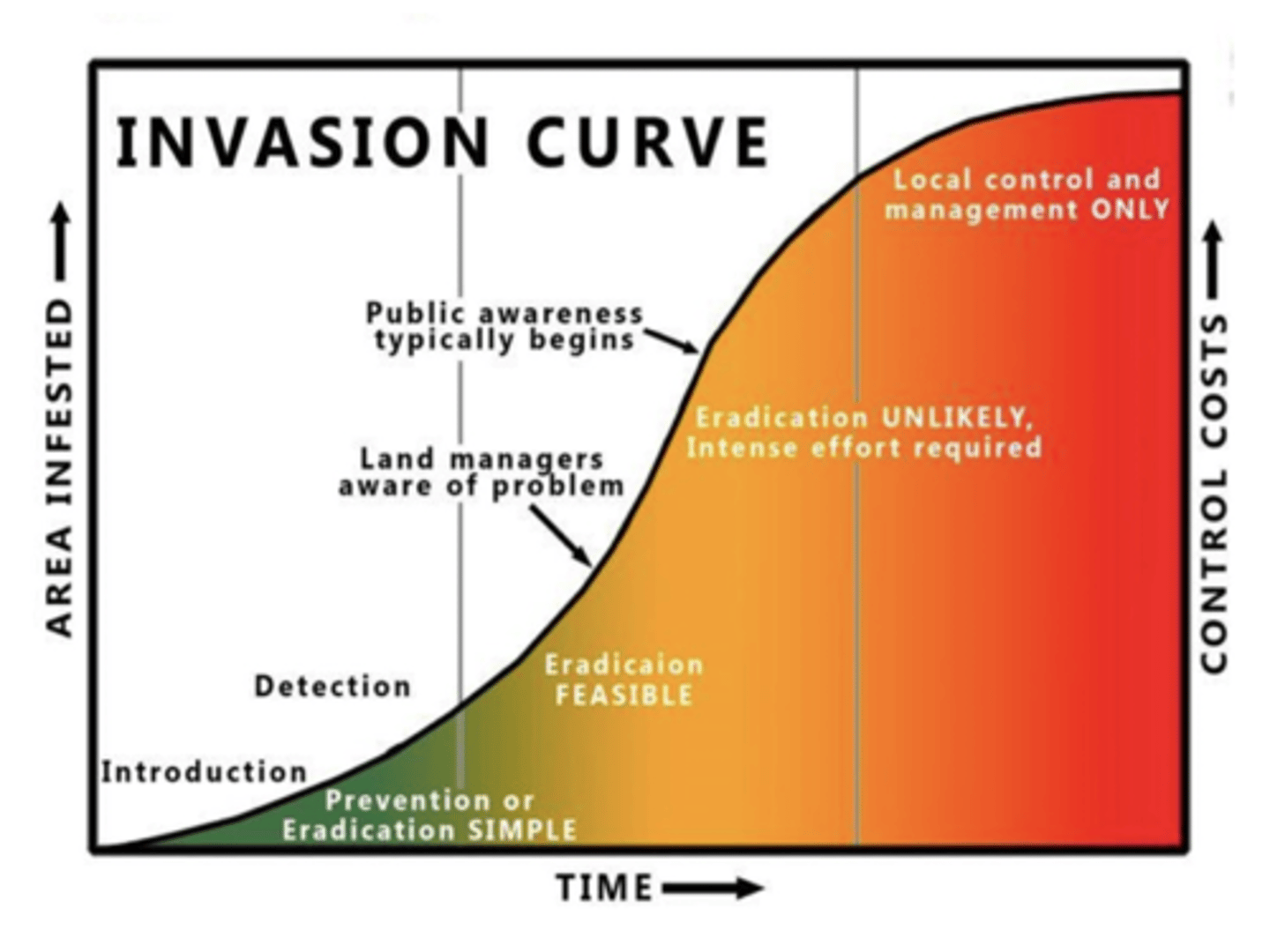
Invasive species exponential growth example

Introduction of rabbits in Australia

○ 1859 a European introduced 12 pairs

○ In 1865, 20,000 rabbits were killed on the ranch

○ By 1900, several hundred million rabbits over most of the continent

Invasive Species and Exponential Growth

Logistic growth model

Limiting factors are environmental factors that restrict

population growth

Introduces a parameter, K

K

maximum population size a particular environment can sustain

Logistic growth model formula

dN/dt = rN (1 - N/K)

Logistic model assumptions

Assumes conditions are uniform and K is constant

Assumes that populations adjust instantaneously to

growth and smoothly approach K

time lag

results from differences in the availability of resources and the time of reproduction

increase the population growth rate over the ordinary logistic - can overshoot k

The length of the time lag might vary from 0 to 3 time

periods in extreme conditions - cycles can be seen for discrete breeders

time lag equation

If there is a time lag of length τ between the change in

population size and its effect on population growth rate,

then the population growth at time t is controlled by its

size at some time in the past, t- τ

dN/dt = rN (1 - N(t-τ)/K)

Density-Dependent Factors

mortality increases as density increases

Density-Dependent Factors example

Where patches of flower heads contain a greater number of fly larvae host plants, a greater proportion were parastized by wasps

Mortality equation

Mortality is sometimes expressed in terms of killing

power:

Killing power = log N (t) - log N(t+1)

Where N(t) is the population size before it is subject to

the mortality factor and N (t+1) is the population size

afterward

killing power example

For oak winter moth pupae on the forest floor, the killing

power of pupal predators acted in a density-dependent manner over time

Examples of density-dependent regulation factors

mortality from limited space/overcrowding

mortality from limited food

predators

parasites and diseases

Density-Independent Factors

mortality is not affected by density

extreme weather events

inverse density-dependent factors

mortality decreases as density increases

In the real world, a small population is extremely vulnerable to extinction

Below a certain critical threshold, instead of increasing, the population can spiral into a steep decline

- Stochastic and deterministic causes; abiotic and biotic

Allee effects

Decline in either reproduction or survival under conditions of low population density

Population Viability Analysis

A method of predicting whether or not a population will persist.

can find chance of going extinct

can find what population size will be less likely to go extinct

Viability of a population

○ Risk of extinction

○ Chance of recovery

○ Expected time of extinction

Viability predicted based on

Demographic data (censuses, m-r, surveys, observations of life history and p/a data)

Assessment of extinction probabilities that includes

○ Life tables

○ Population rates of increase

○ Intraspecific competition

○ Density dependence

○ K

○ Metapopulation structure

Minimum viable population

One that will give at least 95% p(persistence) for 100 years despite the foreseeable effects of demographic,

environmental, and genetic stochasticity and natural

catastrophes

Population Viability Analysis examples

bay checkerspot butterfly, african elephant

Allee effects

Logistic growth model