Bioinfomatics Study Guide Exam 2

5 Stages of Phylogenetic Analysis:

• selection of sequences: BLAST search results, protein families from Pfam, NCBI HomoloGene etc

• multiple sequence alignment of homologous protein or nucleic acid sequences

• specifying models of nucleotide or amino acid substitution

• tree building: distance-based methods, max parsimony, max likelihood & Bayesian inference

• tree evaluation

Distance-based methods:

analyze pairwise sequence alignments & use the distances to infer the relationships between all the taxa

• UPGMA (unweighted-pair group method with arithmetic mean)

• Neighbor-joining

Maximum parsimony:

a character-based method in which columns of residues are analyzed to identify the tree with the shortest overall branch length that can account for the observed character differences

Maximum likelihood & Bayesian inference:

model-based statistical methods to infer the best tree that can account for the observed data

Popular Software Tools for Phylogeny:

• MEGA (molecular evolutionary genetics analysis)

• PHYLIP (PHYLogeny inference package)

• PAUP (phylogenetic analysis using parsimony)

• TREE-PUZZLE (max likelihood method)

• MrBayes (bayesian estimation of phylogeny)

__ comprises all the RNA transcripts synthesized by an organism

transcriptome

Proteome:

the entire set of proteins translated

Metabolome:

refers to the sum total of all the low-molecular-weight metabolites

Experimental approaches of gene expression

• DNA microarrays

• RNA-seq

“Large p, small n” problem:

gene expression studies typically measure the expression levels of 10s of 1000s of genes in only a few samples

DNA microarrays & RNA-seq have been widely used to __

identify which genes are significantly up/down-regulated (differently expressed)

Hypothesis testing:

inferential statistics; assign confidence to the discovery of regulated genes

Exploratory statistics:

define distances between genes; perform unsupervised analyses (clustering, PCA)

Classification:

perform supervised analyses (linear discriminants, support vector machines)

Affymetrix platforms for human microarrays

• HG-U133 Plus 2.0:

  • 54, 120 probe sets

  • multiple probe sets for some genes

• HG-U133A:

  • 27, 722 probe sets

  • well-characterized genes (RefSeq)

• HG-U133B:

  • 22, 577 probe sets

  • representing EST clusters

In RNA sequencing, lower # of reads = __

lower expression

In RNA sequencing, higher # of reads = _

higher expression

Sample-level/global normalization:

to remove the systemic bias in the data so that meaningful biological comparisons can be made

• unequal quantities of starting RNA

• experimental/technical variations

Normalization is based on the assumption that __

the total intensity distribution is comparable between 2 samples & the expression of a subset of genes is assumed to be constant

Why do we use sample-level/global normalization?

to allow valid cross-sample comparison & to minimize non-biological variation

Sample-level/global normalization method:

• normalize all values for a sample so that median = 1

• normalize to positive control genes

• normalize to a constant value

Gene-level normalization:

rescales all genes to the same normalized value range & thus enables comparison of relative expression levels

Z transformation:

for each gene, calculate the z scores of the expression values

z_xi = (x_i - ^-x^-) / σ_x

__ normalizes distribution

log transformation

In RNA-Seq Data Preprocessing and Normalization, experimental design needs to include __

sufficient replicates to measure biological variablity

RNA-Seq Data Preprocessing and Normalization steps:

• experimental design

• RNA acquisition

• data acquisition

• mapping

• summarization

• normalization

RPKM/FPKM (Reads/Fragments per Kilobase of transcript per Million mapped reads):

• counts are first normalized for sequencing depth

• counts are then normalized for gene length

• FPKM for paired-end RNA-seq data

TPM (transcript per million):

• proposed as an alternative to RPKM/FPKM

• technology-independent measure of expression

Mapping software used to align unmapped reads to a reference genome is __ in RNA-Seq Data Preprocessing and Normalization

Tophat

Mapping software used to align millions of short reads to a reference genome is __ in RNA-Seq Data Preprocessing and Normalization

Bowtie

Advantages of RNA-seq

• not limited to detection of known gene transcripts

• little to no background signal

• can detect large dynamic range of expression levels

RNA-seq can reveal information about __ resulting from alternative splicing methods

different transcript isoforms

RNA-seq can be used to discover __ such as lncRNAs

novel transcripts

Bowtie:

extremely fast, general purpose short read aligner

Tophat:

fast splice junction mapper for RNA-seq reads; aligns reads to the genome using Bowtie & discovers splice sites

Cufflinks:

assembles transcripts

Cuffcompare:

compares transcript assemblies to annotation

Cuffmerge:

merges 2 or more transcript assemblies

Cuffdiff:

finds differentially expressed genes and transcripts & detects differential splicing and promoter use

Bioconductor

an open source software project, based on R, to provide tools for the analysis of high-throughput genomic data

GEO2R

a web-based tool for comparing two or more groups of Samples in a GEO Series to identify differentially expressed genes. performs comparisons on original submitter-supplied processed data using R packages from Bioconductor

MeV (MultiExperiement Viewer)

a versatile tool (web-based or standalone) for expression data analysis, with sophisticated algorithms for statistical analysis, clustering, visualization, and classification

Experimental design

Compare normal vs diseased tissue, cells ± drug, early vs late development

RNA preparation

Isolate total RNA or mRNA

Microarrays

Fluorescently label cRNA samples and preprocessing (normalization, scatter plots)

RNA-seq

Make cDNA library for each sample and and align reads to genome or gene models; assemble transcripts

Inferential statistics

Identify significant regulated transcripts e.g. using ANOVA

Exploratory analyses

Scatter plots, principal components analysis

Other analyses

Classification, co-regulated genes

Biological confirmation

Independently confirm that genes are regulated e.g. by RT-PCR

Deposit data in a database

GEO, ArrayExpress, ENA, SRA

Fold change

Uses a fold change threshold (e.g., 2-fold) to select genes; does not take into account the biological and experimental variability

Statistical tests

Such as t test and ANOVA; require a number of replicates for each condition

Bonferroni correction

Bonferroni correction:

• Set the significance cutoff, p' = α / N, where α is the false positive rate, and N is the number of genes

• If you have 10,000 genes in your dataset, with 5% of false positives, p' = 0.05 / 10000 = 0.000005 (5 E - 6)

• Calculate the adjusted p value: Padjusted = p * N

False Discovery Rate (FDR)

• Rank all the genes by significance (p value) so that the top gene has the most significant p value

• Start from the top of the list, and accept the genes if: p less than or equal to (i/N)q

• i = the rank of the gene in the list, N = the number of genes in the dataset, q = the desired FDR

ANOVA (ANalysis Of VAriance)

Used to find significant genes in more than two conditions

Clustering Analysis

Divide a dataset into a few groups (clusters)

Homogeneity

Objects in the same cluster are similar to each other

Seperation

Dissimilar objects are placed in different clusters

Expression Vector

Each gene can be represented as a vector in the N-dimensional hyperspace, where N is the number of samples

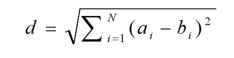
Euclidean distance

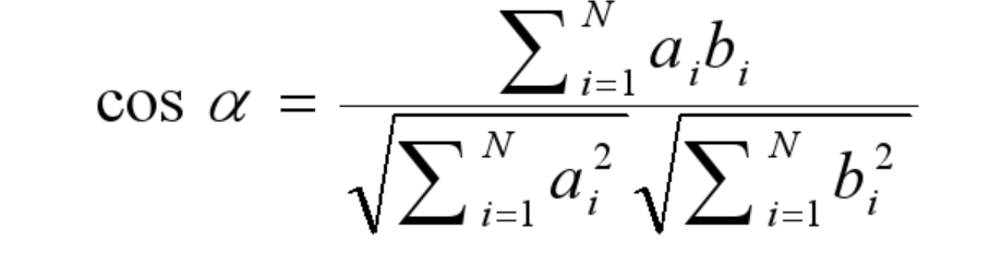
Vector angle

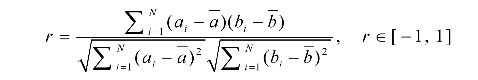
Pearson’s correlation coefficient

Initialization (Hierarchical Clustering Algorithm)

Each object is a cluster

Iteration (Hierarchical Clustering Algorithm)

Merge two clusters which are most similar to each other until all objects are merged into a single cluster

Hierarchical Clustering

Results are often visualized using a tree (called dendrogram) with color-coded gene expression levels. Can be applied to genes, samples, or both

Initialization (k-Means Clustering)

User-defined k (# clusters) randomly place k vectors (called centroids) in the data space

Iteration (k-Means Clustering)

Each object is assigned to its closest centroid re-compute each centroid by taking the mean of data vectors currently assigned to the cluster until the cluster centroids no longer change

Self-Organizing Map (SOM)

• The user defines an initial geometry of nodes (reference vectors) for the partitions such as a 3 x 2 rectangular grid

• During the iterative “training” process, the nodes migrate to fit the gene expression data

• The genes are mapped to the most similar reference vector

Gene Co-expression Network Analysis

• A gene co-expression network is an undirected graph, in which each node is a gene, and each edge represents a significant co-expression relationship between two nodes

• It can be constructed by looking for pairs of genes which show a similar expression pattern across various samples

• Does not attempt to infer the causal relationships between genes, and thus is different from a gene regulatory network

How to Assess Whether a Gene Ontology (GO) Term Is Enriched in a Gene List?

Compare gene with one already saved in the database

Database for Annotation, Visualization, and Integrated Discovery (DAVID)

• Can be used to extract biological meaning from large lists of genes

• DAVID’s functional enrichment analysis of a gene list is based on a modified version of the Fisher’s exact test

How to Represent a Promoter Motif?

• Multiple sequence alignment

• Consensus: e.g., TATAAAA (the TATA box)

• Position Weight Matrix (PWM): relative frequencies of nucleotides at different positions

• Sequence logo: information content of each site (a measure of intolerance for substitution)

PWM Representation of a Motif

• A motif is assumed to have a fixed width, W

• In the PWM, pnk is the probability (relative frequency) of nucleotide n in column k

• Background probability: pn0 is the probability of n in the background (i.e., outside the motif)

• Equal distribution: pA0 = pC0 = pG0 = pT0 = ¼

Pattern matching

• Scanning a nucleotide or protein sequence for matches to a known pattern

• How to get better sensitivity and specificity is the major consideration

Pattern discovery

• Given a set of sequences, discovering a pattern that is shared by the sequences.

• It is unknown in advance about what is the pattern

• Using search or learning approaches

• A much harder problem than pattern matching

Multiple EM for Motif Elicitation (MEME)

• Widely used for discovery of DNA and protein sequence motifs

• It is based on the Expectation Maximization (EM) algorithm with several extensions

• MEME is now complemented by the GLAM2 algorithm which allows discovery of motifs containing gaps

Protein Structure

• Proteins are very complex molecules with diverse functions

• Levels of protein structure:

1. Primary structure

2. Secondary structure

3. Tertiary structure

4. Quaternary structure

• Simple images highlighting specific features are useful:

1. Space-filling models

2. Ribbon cartoon models

Protein Primary Structure

• Amino acid sequence of a polypeptide chain

• 20 amino acids, each with a different side chain (R)

• Peptide units are building blocks of protein structures

• The angle of rotation around the N−Cα bond is called phi, and the angle around the Cα−C′ bond from the same Cα atom is called psi

Protein Secondary Structures

• Local structures as a result of hydrogen bond formation between the carbonyl and N-H groups in the polypeptide backbone (backbone interactions)

• Types of secondary structures:

1. Alpha helix

2. Beta sheet

3. Loop or random coil

• Secondary structure formation is influenced by several properties (e.g., size and charge) of amino acid side chains

Alpha Helix

• Most abundant secondary structure

• 3.6 amino acid residues per turn, and hydrogen bond formed between every fourth residue

• Proline (with no N-H group) and glycine (too small) do not foster alpha helix formation

Beta Sheet

• Two or more polypeptide chains line up side by side

• Hydrogen bonds formed between adjacent strands

• The chain directions can be same (parallel sheet), opposite (antiparallel), or mixed

• Antiparallel beta sheets are more stable than parallel beta sheets

Loop or Coli

• Regions between alpha helices and beta sheets

• Various lengths and 3D configurations

• Often functionally significant (e.g., part of an active site)

Supersecondary Structures (Motifs)

• Many proteins contain supersecondary structures (motifs) with combinations of alpha-helices and beta-sheets

• In the beta-alpha-beta motif, two beta-strands and one alpha-helix are connected by loops

Protein Tertiary Structure

• The unique three-dimensional structure formed by a globular protein

• Stabilized by hydrophobic interactions, hydrogen bonds, and other interactions

Important Features of Tertiary Structures

• Many polypeptides fold in a way to bring distant amino acid residues in the primary structure into close proximity

• Globular proteins are compact because of efficient packing as the polypeptide folds

• Enough hydrophobic surface must be buried, and the interior must be sufficiently packed

• Buried polar atoms must be hydrogen-bonded to other buried polar atoms

• Large globular proteins often contain several compact units called domains

Protein Domains

• Structurally independent segments that have specific functions

• The core 3D structure of a domain is called a fold

• A certain type of 3D arrangement of secondary structures

• Domains are classified on the basis of their core structure:

• Alpha: composed exclusively of alpha - helices

• Beta: consists of antiparallel beta -strands

• Alpha/beta : contains various combinations of alpha -helices and beta -strands

Protein Quaternary Structure

• Two or more polypeptide chains (subunits) form a larger protein complex

• Protein subunits are often held together by non-covalent interactions, including hydrophobic interactions (most important), electrostatic interactions, and hydrogen bonds

• Important for understanding protein-protein interactions

Unstructured Proteins (Regions)

• Some proteins are partially or completely unstructured

• Unstructured proteins (regions) are referred to as intrinsically disordered proteins (regions)

• Over 30% of eukaryotic proteins are partially or completely disordered and have a variety of functions

• The disordered segments (e.g., KID domain of CREB) may be involved in searching out binding partners

X-Ray Crystallography

• Basic steps: Expression/purification, Crystallization, X-ray diffraction, Structure solution

• Advantages: High-resolution structures, large protein complexes or membrane proteins

• Disadvantages: Requirement for crystals, molecules in a solid-state (crystal) environment

Nuclear Magnetic Resonance (NMR)

• Reveals information on the distances between atoms in a molecule, and these distances can be used to derive a 3D model of the molecule

• Advantages: No requirement for crystals, proteins in a liquid state (near physiological state)

• Disadvantages: Limited by molecule size (up to 30 kD), inherently less precise than X-ray crystallography, membrane proteins may not be studied

Cryogenic Electron Microscopy (Cryo-EM)

• A beam of electrons is fired at a frozen protein solution. The emerging scattered electrons pass through a lens to create a magnified image on the detector, from which their structure can be worked out

• Advantages: No crystal requirement for large complexes, structure remains in native state (no dehydration)

• Disadvantages: Relatively low resolution (but improving), 3D structure reconstruction from 2D images

Protein Data Bank (PDB)

• Established at Brookhaven National Laboratory in 1971, initially with seven structures

• Was moved to the Research Collaboratory for Structural Bioinformatics (RCSB) in 1998

• The RCSB PDB (https://www.rcsb.org/) has been the primary repository for 3D structural data of proteins, nucleic acids, and complexes

• The Worldwide PDB (wwPDB, http://www.wwpdb.org/) was formed in 2003 to maintain a single PDB archive of macromolecular structural data

RCSB PDB

• PDB supports services for structure submission, search, retrieval, and visualization

• By 3/6/2026, PDB contains 250,441 experimental structures and 1,068,577 computed structure models

Search RCSB PDB

• Basic search using a PDB identifier or keywords: A PDB ID consists of one number and three letters (or numbers) (e.g., 4HHB for a human hemoglobin structure; pdb_00004hhb)

• Advanced search with specific attributes or data types, sequence search (BLAST/PSI-BLAST, or FASTA)

Protein Structure File Formats

PDB supports the download of protein structural data in the following text file formats:

• PDB file format: outdated but human-readable

• PDBx / mmCIF: simple and consistent data representation for exchanging and archiving structural data, used by PDB to store its files

• PDBML / XML: a modern and robust file format

Access to Structures through NCBI

• MMDB (Molecular Modeling Database)

1. Structures obtained from PDB

2. Data in NCBI’s ASN.1 format

3. Integrated into NCBI’s Entrez system

• Cn3D (“see in 3D”): NCBI’s protein structure viewer

• VAST (Vector Alignment Search Tool): for direct comparison of 3D protein structures to identify structural neighbors

RasMol and RasTop

• RasMol: An open-source software package, which was a breakthrough in 3D

structure visualization. It is widely used to view 3D protein structures.

• Structure file formats supported by RasMol:

1. PDB file format

2. mmCIF file format

• RasTop: Provides a graphical user interface to RasMol

Other 3D Visualization Tools

• Jmol: An interactive web-browser Java applet to view chemical structures in 3D, and JSmol is a JavaScript-based extension

• Cn3D: Can be used for interactive exploration of 3D structures, sequences, and alignments

• Swiss-Pdb Viewer (DeepView): Probably the most powerful freely available molecular

• modeling and visualization package. Supports homology modeling, site-directed mutagenesis, structure superposition, etc.

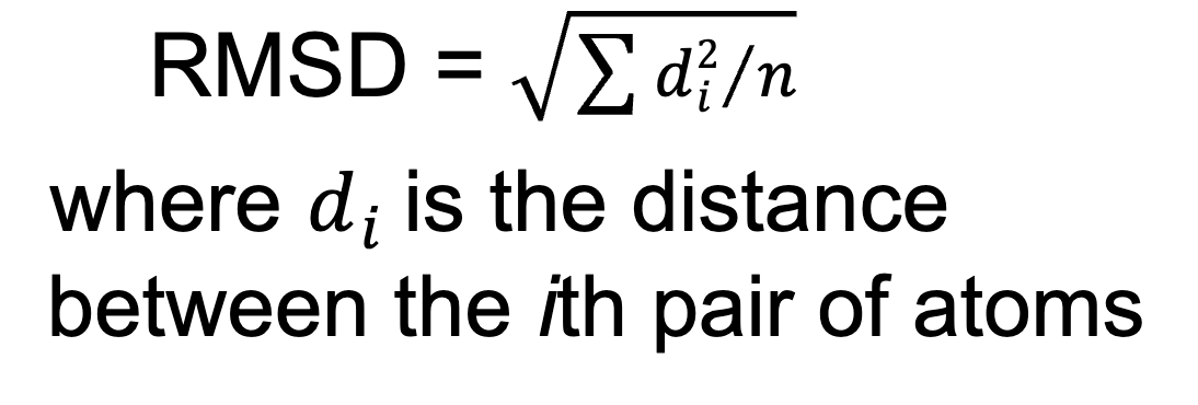
Root-mean-square deviation (RMSD)