PHYS 421 Midterm 2

The three interpretations of quantum indeterminacy

Realist: particle had definite value all along, QM is incomplete. Orthodox (Copenhagen): no definite value until measured, collapse is real. Agnostic: the question is meaningless since it can't be tested

Copenhagen interpretation

The particle does not have a definite value before measurement. The act of measuring forces it into a definite state (wave function collapse). This is the interpretation experiments have confirmed

Realist interpretation

QM is incomplete — a hidden variable carries the true state of the particle before measurement. Realism also typically implies locality

Singlet state

|ψ⟩ = (1/√2)(|+⟩₁|−⟩₂ − |−⟩₁|+⟩₂).

Arises when a spin-0 particle decays into two particles; total spin must stay zero so the two spins are always opposite.

Spooky action at a distance

Einstein's phrase for the apparent instantaneous influence of Alice's measurement on Bob's distant particle. When Alice collapses her particle to spin-up, Bob's instantly becomes spin-down no matter how far apart they are.

EPR argument

Einstein, Podolsky, and Rosen argued that the perfect correlations between distant particles prove hidden variables must exist — particles carry pre-programmed instructions from decay, preserving locality.

Post-measurement collapsed state (EPR)

If Alice measures particle 1 and gets +ℏ/2, the state collapses to |+⟩₁|−⟩₂. The projector ₁⟨+| kills the second term via orthogonality, leaving Bob's particle definitely spin-down

General recipe for post-measurement state

|measured eigenstate⟩ · ⟨measured eigenstate|ψ⟩. The bra gives the component (a number); the ket puts you back in state space. Same structure as projecting a vector onto an axis.

Bell's inequality (spin setup)

For any local hidden variable theory, 𝒫same ≤ 4/9. Derived by exhausting all possible hidden instruction sets across three axes each 120° apart and showing the same-result fraction can never exceed 4/9.

QM prediction for 𝒫same in Bell test

𝒫same = 1/2. Using sin²(θ/2) with θ = 0° for 1/3 of measurements and θ = 120° for 2/3: (1/3)(0) + (2/3)(3/4) = 1/2. This exceeds the hidden variable bound of 4/9.

This prediction demonstrates the violation of Bell's inequality, indicating non-local correlations in quantum mechanics.

Significance of Bell inequality violations

No local hidden variable theory can be correct. Particles don't carry pre-programmed answers. The Copenhagen interpretation is confirmed. Awarded the Nobel Prize in Physics in 2022.

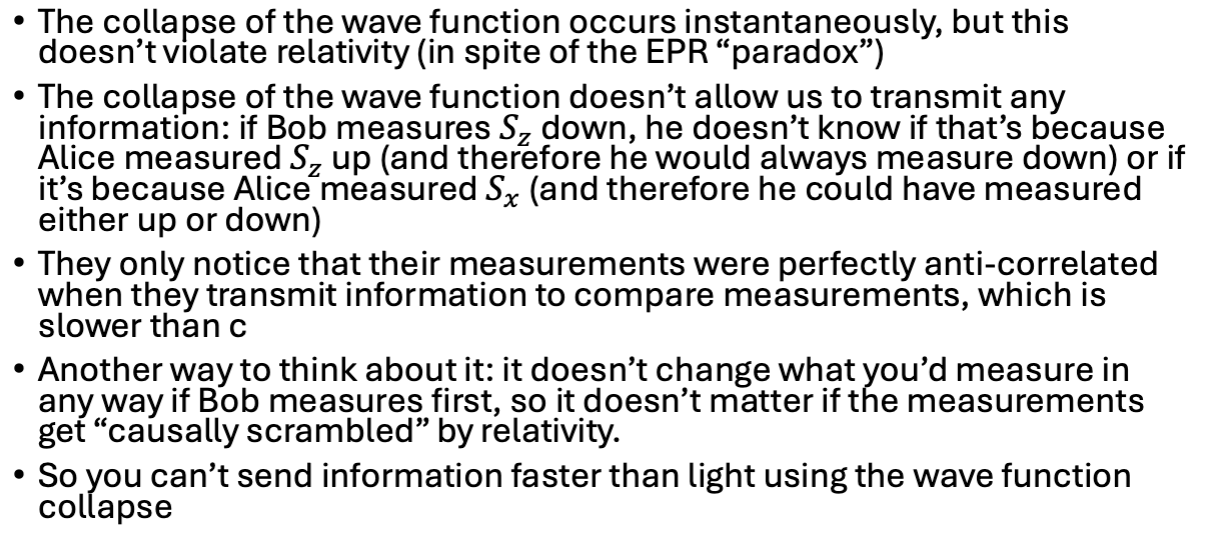
Wave function collapse and special relativity

Collapse is instantaneous but does not violate relativity. Bob's outcome looks random regardless of what Alice does — the anti-correlation is only visible when they compare results classically, which is limited to the speed of light.

Neutrino oscillations and mass

Flavor eigenstates (production/detection) and mass eigenstates (time evolution) are different bases. If neutrinos were massless there would be no oscillation. Non-zero mass creates energy differences that drive flavor-changing probability, described by Rabi's formula

why doesnt wave functino collapse violate relativity

The instantaneous nature of wave function collapse doesn't transfer information faster than light, retaining consistency with relativity. Observers perceive randomness in outcomes until classic comparison occurs, constrained by light speed.

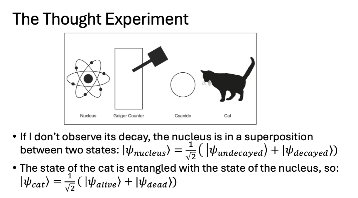
schrodingers cat set up

In the Schrödinger's cat thought experiment, a cat is placed in a sealed box with a radioactive atom, a Geiger counter, and a vial of poison. If the atom decays, the Geiger counter triggers the release of the poison, leading to the cat being simultaneously alive and dead until observed.

energy eigenvalue equation

Hamiltonian operator = H^

H^ |E_i> = E_i |E_i>

how is hamiltonian related to potential energy

hamiltonian determines the energy states through energy eigenvalue equation H^ |E_i> = E_i |E_i>

how to find quantum mechanical hamiltonian operator

find classical form of energy and replace physical observables with their quantum mechanical operators

ex: moving particle in classical mechanics has energy = K + U

→ E_classical = p_x²/2m + V(x)

→ posiiton x and momentm p are primary physical observables in QM so: H^ = p^_x² / 2m + V(x^) (carrots/hats distinguish operators from variable)

wave functions

spatial functions we use to represent quantum states (more convenient to represent abstract quantum states than kets)

|psi> = psi(x)

collection of numbers that represents the quantum state vector in terms of position eigenstates (in the same way that a column vector used to represent a general spin state is a collection of numbers taht represents quantum state vector in terms of spin eigenstates)

psi(x) in bra ket notation

<x | psi>

position representation

|psi> = psi(x)

we are using position eigenstates as preferred basis

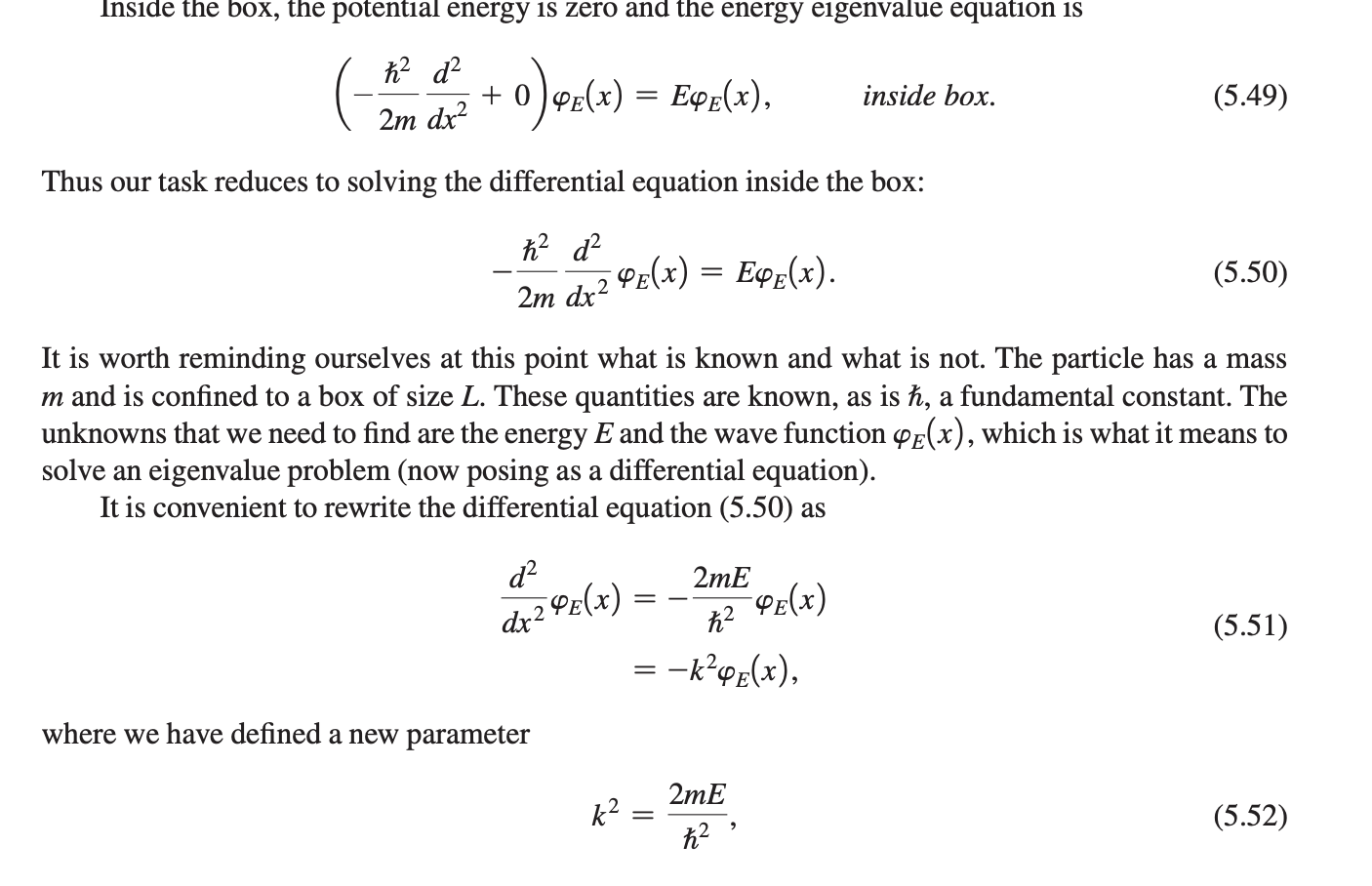
how do we write wavefunctions of energy eigenstates

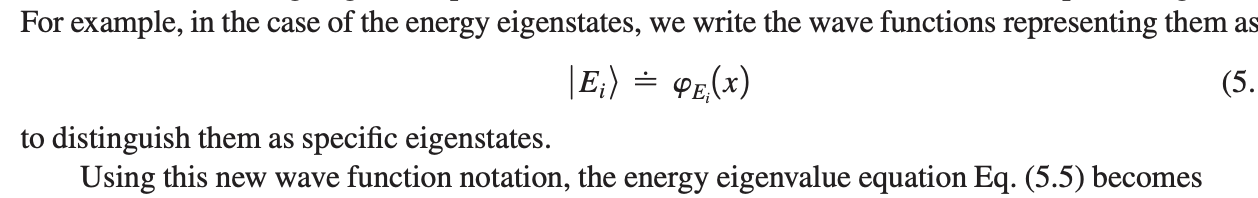
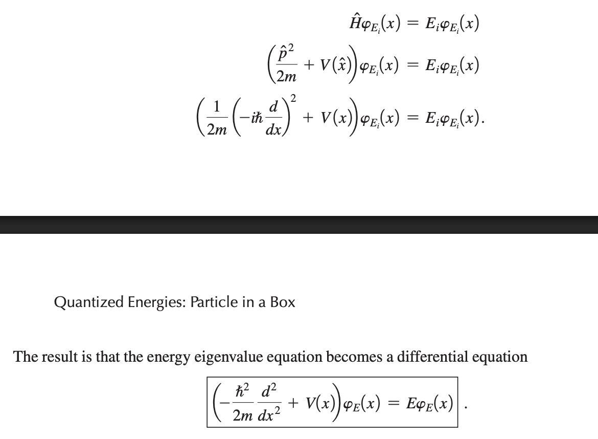
energy eigenvalue equation in terms of wave functions

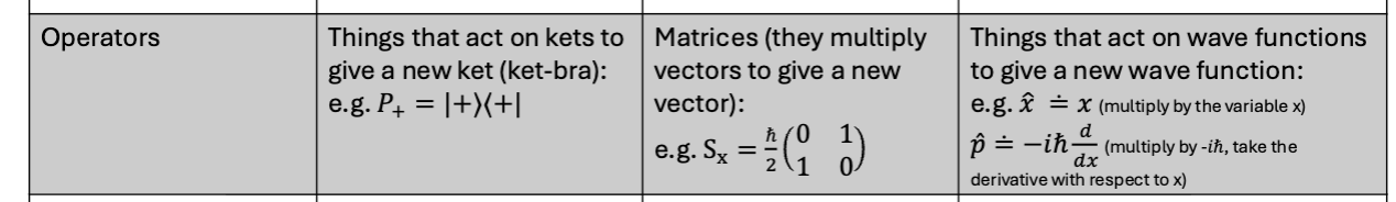
how do we define position and momentum operators

x^ = x

p^ = –i hbar d/dx

momentum operator is representation by application of a derivative with respect to position, has factor –i hbar to get dimensions correct and to ensure measurements are real (NOT imaginary)

solve energy eigenvalue equation using wave functions and position/momentum operator definitions

solving this eqn gives eigenstates and eigenvalues (in matrix rep we found eigenstates and eigenvals by diagonalizing matrix of H)

when using wave function approach: operator equations turn into ___

DIFFERENTIAL EQUATIONS

bound state

a particle interacting with its environemtn or another particle(s) in a way that binds it into a composite system

particles that have their motion constrained by potential well are in bound states

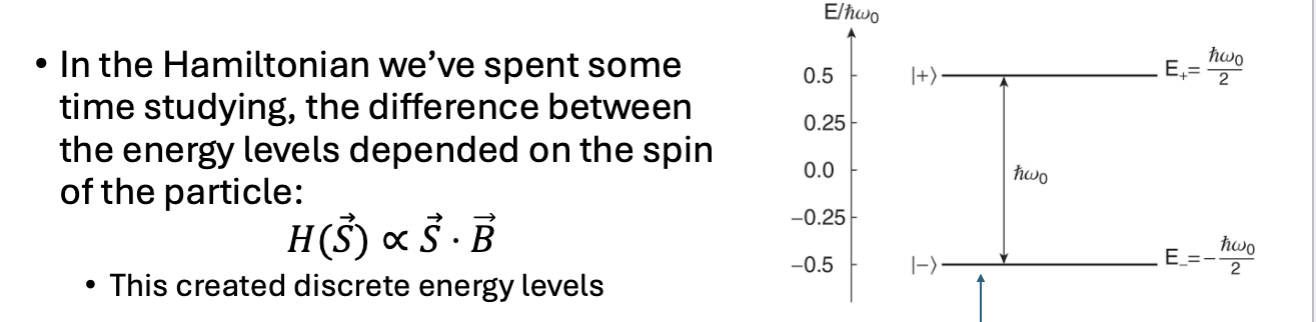
difference bwn energy levels depends on

SPIN of particle

if a charged particle in a stationary state gets perturbed (by a collision, or by shining light on it, etc) it can:

undergo a transition to another stationary state by absorbing energy

how do particle transitions happen in QM like with hydrgen spectrum?

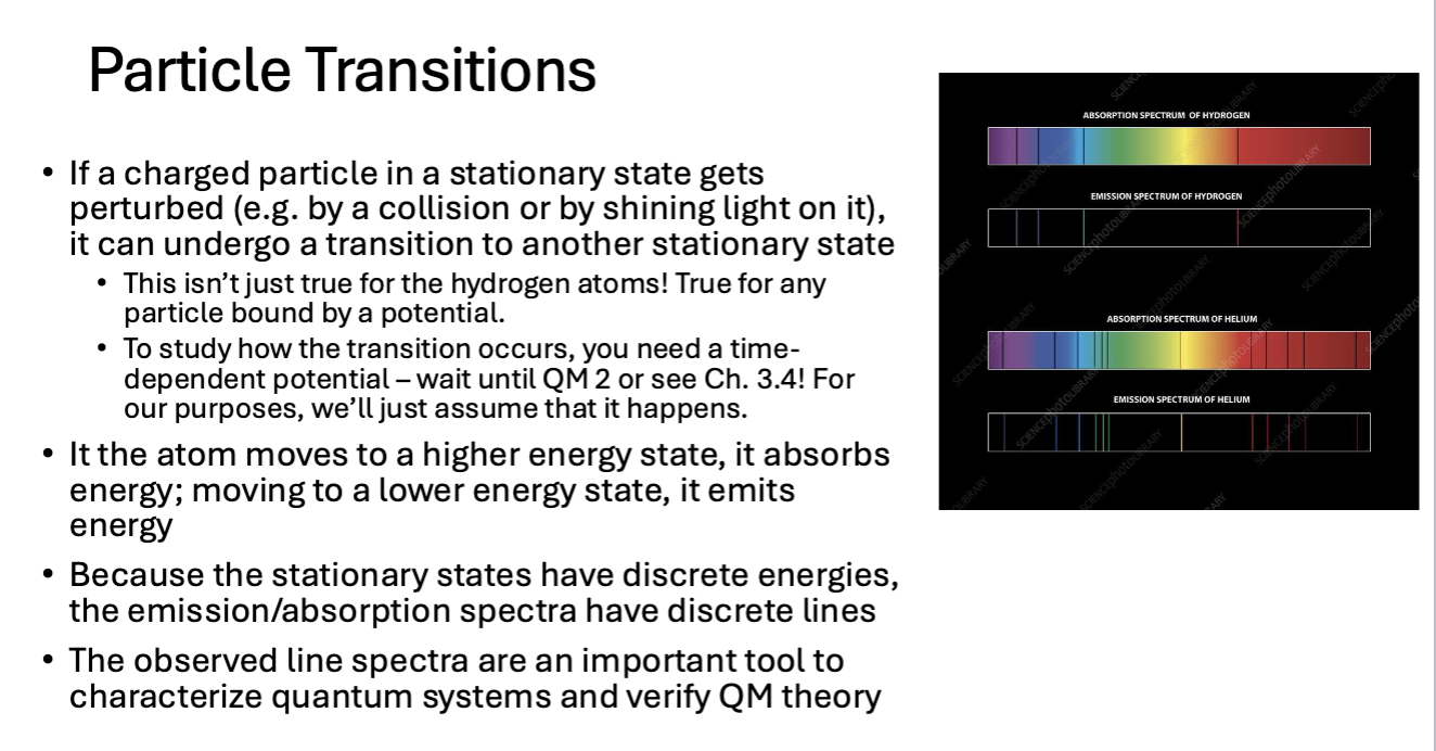
if charged particle in stationary state gets perturbed (absorbs energy) it can undergo transition to another stationary state → atoms moves to higher E state by absorption, lower E state by emission → bc stationary states have discrete energies the abs/emis spectra have discrete lines

criteria to see absorption specgtrum

populate ground state

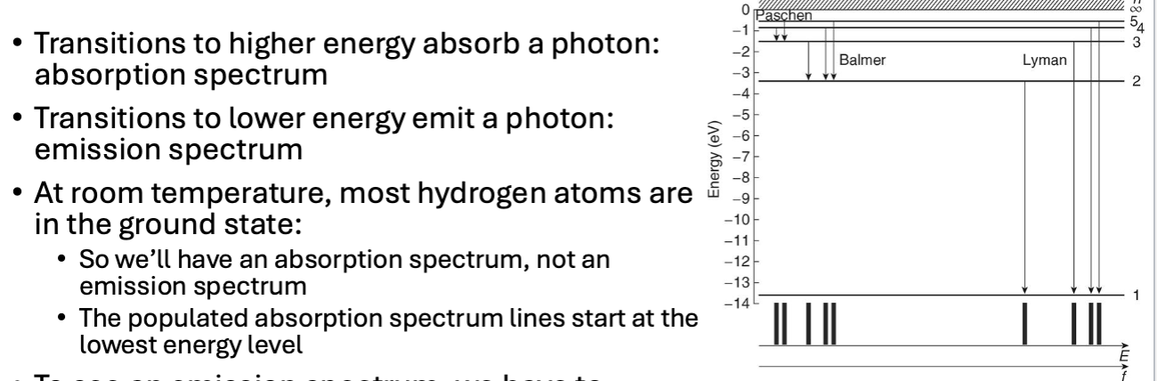
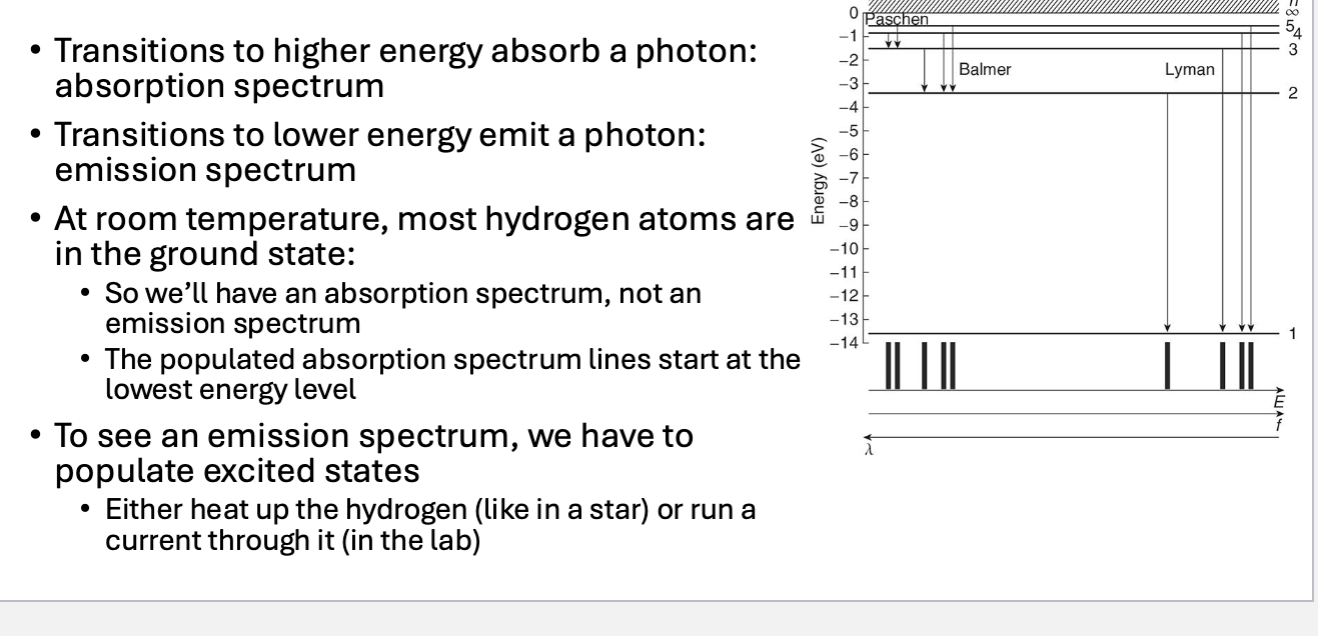
criteria to see emission spectrum

populate excited states

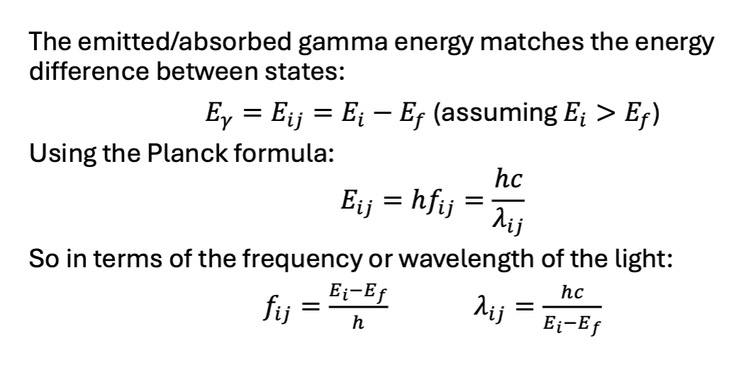
planck formula

shows that emitted/absorbed gamma energy for particle transitions matches the energy difference bwn stationary states

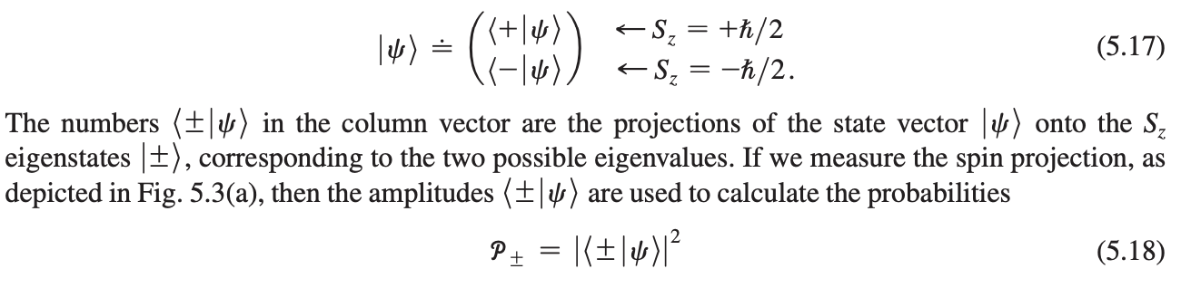
how to calculate probabilities using spin in dirac notation

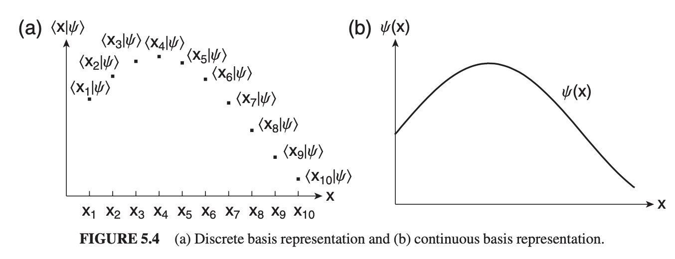
spectrum of eigenvalues of position vs. eigenvalues of spin

physical observable x is NOT qunatized → thus ALL position x values are allowed → so spectrum of eigenvalues of position is continuous

in case of spin S_z only two results were possible → spectrum of eigenvalues of spin is discrete

wave function as a probability amplitude

wavefunction psi(x) is probability amplitude for quantum state |psi> to be measured in position eigenstate |x>

probability density from wave functions

P(x) |psi(x)|²

NOTE: this is P(x) (probability DENSITY) aka a funcion bc wave function is continuous (diff from discrete probabilities from spin)

normalization condition from wave function

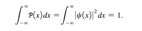
dx has dimensions of length

total integrated probability must be dimensionless → P(x) has dimensions of INVERSE length (thus why it’s a probability DENSITY)

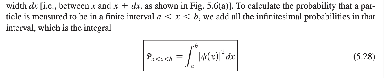
P(x)dx is infinitesimal probability of detecting a particle at position x within an infinitesimal region of width dx

how to calculate probability over a finite interval from wave function

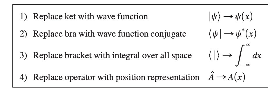
translating bra ket to wave function formulas

1. ket

2. bra

3. bra ket

4. operator

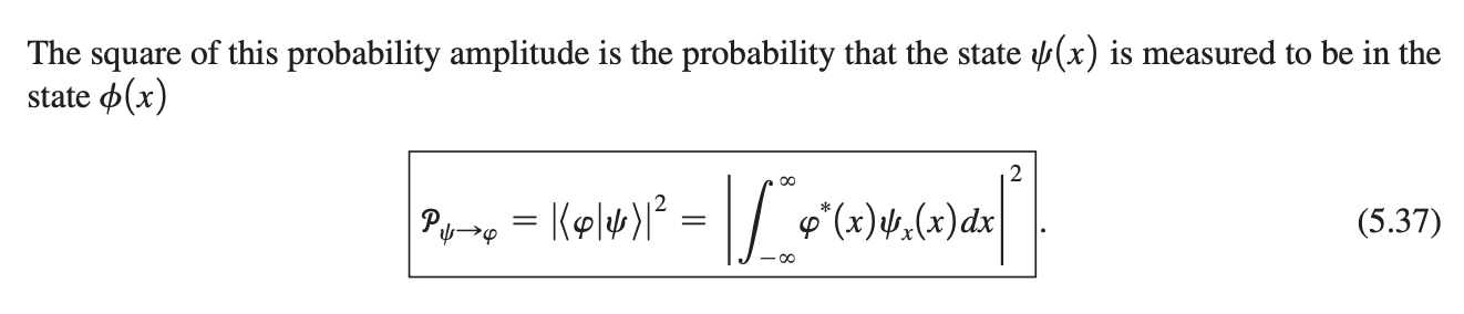
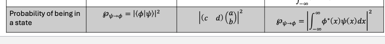
probability the state psi(x) is measured to be in the state phi(x)

how to calculate expectation value of position in wave function notation

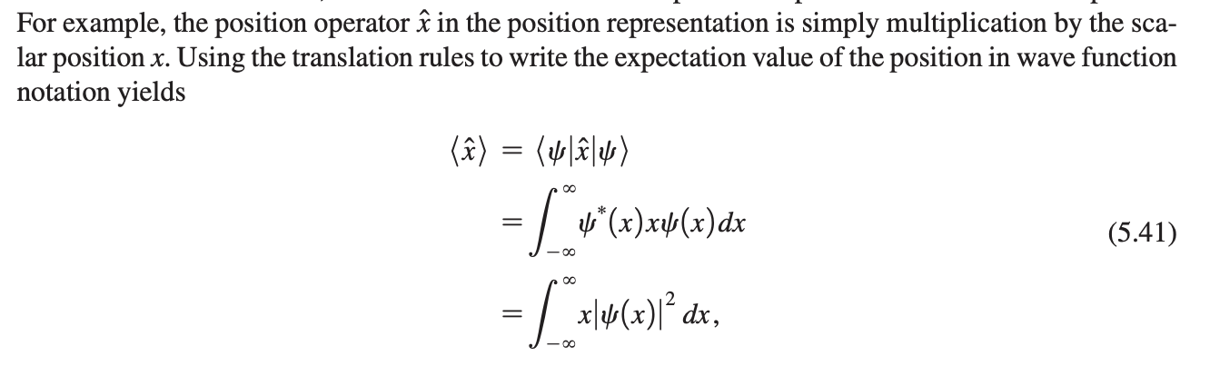
how to calculate expectation value of momentum in wave function notation

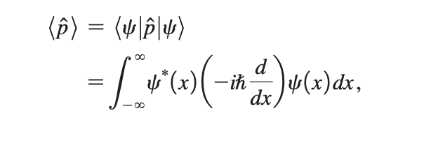
can’t simplify more iwthout knowing wave function

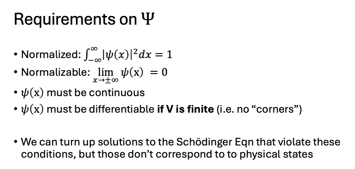
what are conditions for normalizability of wave function

integral from -infinity to +infinity of |psi(x)|²dx MUST converge if has to equal 1 → thus psi(x) MUST go to 0 as x goes to ±infinity

when do we use dirac vs. matrix vs. wave function representations?

dirac: always works

matrix: used for discrete finite sets of eigenstates (ex: S_z)

wave function: used for infinite continuous sets of eigenstates (ex: position rep)

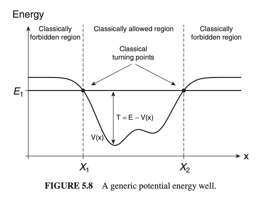
potential well

when potential energy curve V(x) has a minimum → then we say potential energy function is a potential well

A potential well is a region in space where the potential energy is lower than the surrounding areas, causing particles to be trapped and possessing quantized energy levels. In quantum mechanics, this concept is frequently illustrated using solutions to the Schrödinger equation.

kinetic energy of particle in potential well

energy is conserved: total energy = potential + kinetic

• total energy = E

• potential = V(x)

• kinetic = T(x)

T(x) = E - V(x)

where does classically forbidden region come from

In quantum mechanics, the classically forbidden region arises in areas where the potential energy exceeds the total energy of the particle, leading to an absence of classical motion. In these regions, the wave function can still have non-zero values, indicating a probability of finding the particle within these boundaries.

classical particle: kinetic energy cannot be negative so classical particle can’t have T = E-V be <0 (comes from V>E)

classical turning points

The classical turning points are the locations in a potential well where the kinetic energy of a particle becomes zero, marking the boundaries between classically allowed and forbidden regions. At these points, the total energy is equal to the potential energy, resulting in a change in the motion of the particle.

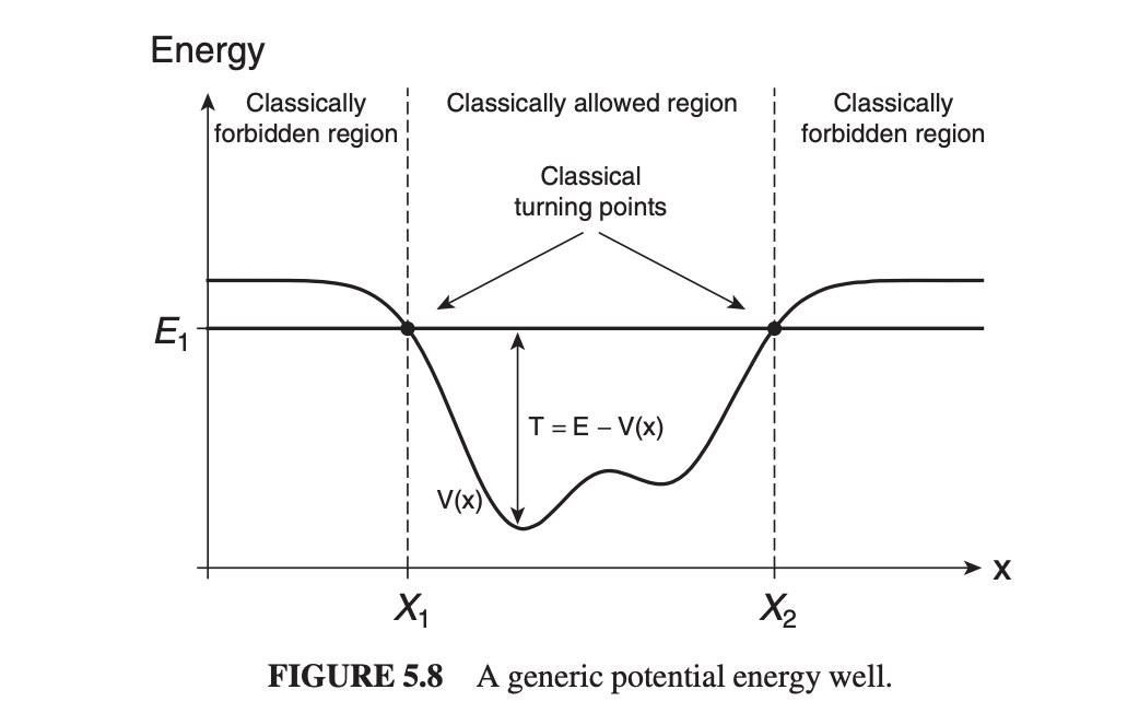
classically allowed vs. forbidden region

The classically allowed region refers to areas in a potential well where the kinetic energy of a particle is positive, allowing for classical motion.

In contrast, the forbidden region is where the potential energy exceeds the total energy, resulting in zero or negative kinetic energy and absence of classical motion.

bound vs. unbound state

particles w motion constrained by potential well are in bound states

particles w energies above top of well do NOT have motion constrained so they are in UNbound states

particle in a box model

A fundamental quantum mechanics model that describes a particle confined to a perfectly rigid and impenetrable box.

The energy levels of the particle are quantized, leading to discrete energy states based on the dimensions of the box.

model: ball bounces bwn 2 perfectly elastic walls:

(1) ball flies freely bwn walls → 0 force on ball when it is bwn walls

(2) ball reflected perfectly at each bounce → infinite force on ball at walls

(3) ball remains in box no matter how large its energy → infinite potential energy outside box

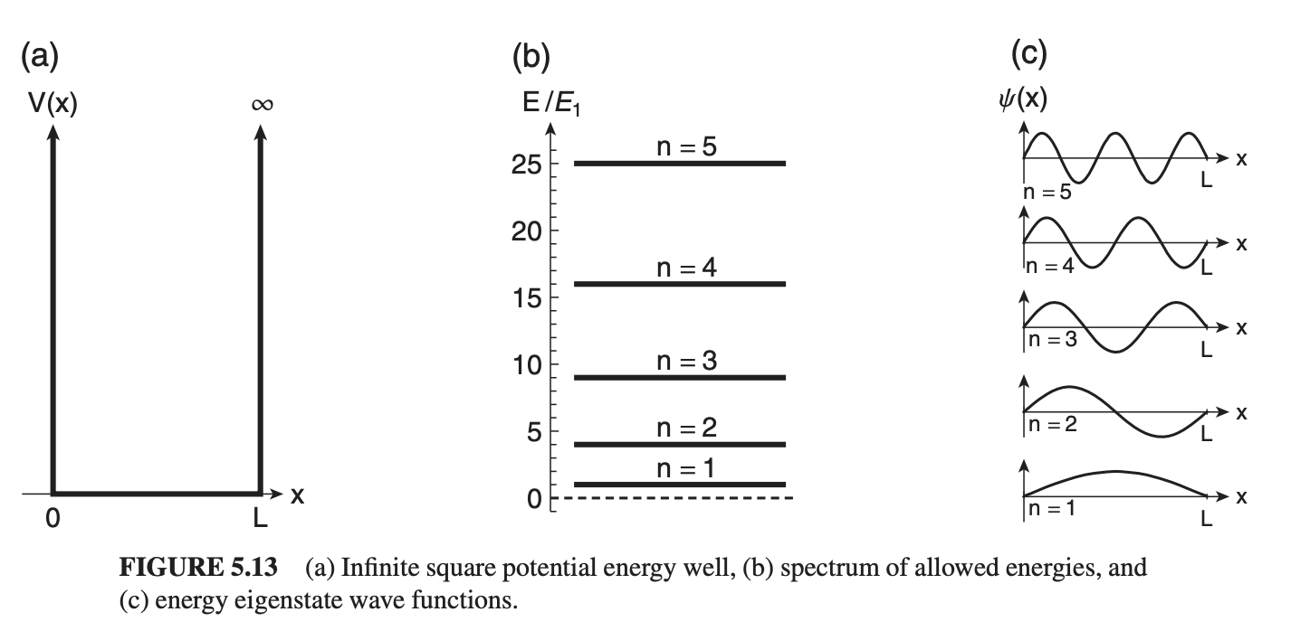
THUS: THIS CREATES INFINITE SQUARE WELL SHAPE:

V(x) = +infinity from x<0, 0 from 0<x<L, +infinity from x>L)

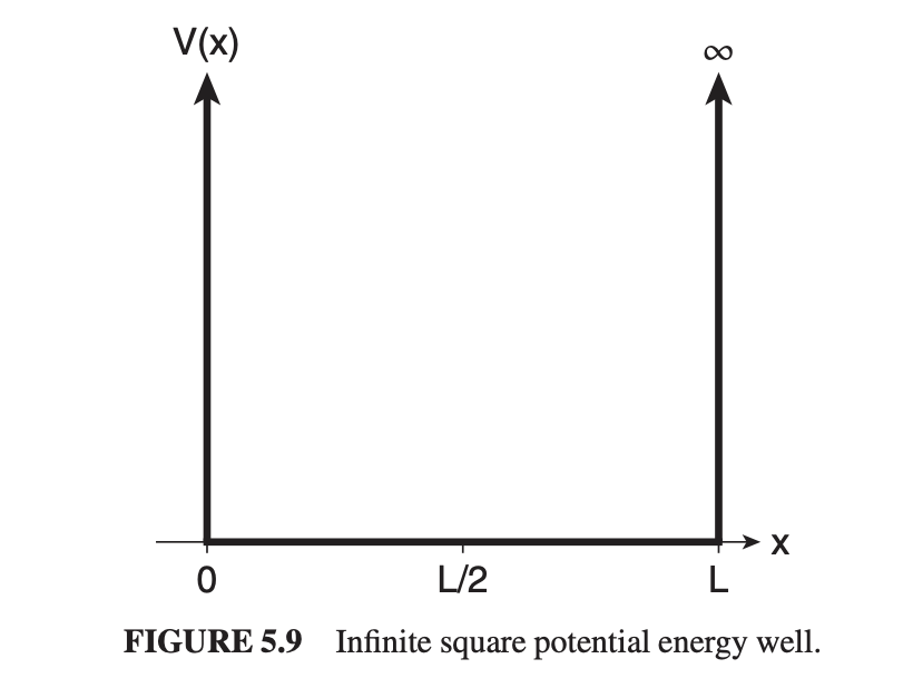
infinite square well and classically forbidden region

The infinite square well represents a quantum mechanical model where a particle is trapped in a box with infinitely high potential barriers, creating classically forbidden regions outside the box where the particle cannot exist. In these regions for the INFINITE well, the potential energy is infinitely high, resulting in no probability of finding the particle → only have to solve energy eigenvalue eqn for where V(x) = 0

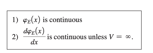
wave function requirements

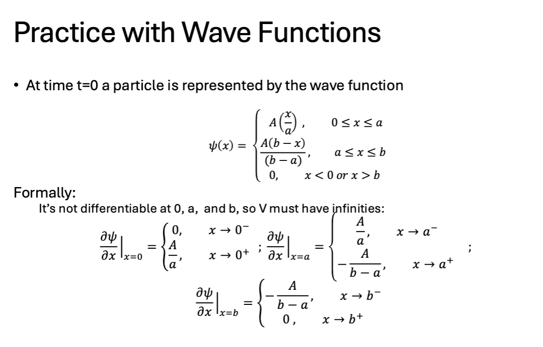
NOTE: psi(x) can ONLY have “corners”/”cusps” where V is infinite → dpsi/dx must be finite unless V is infinite at that point

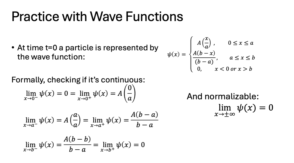
how to check if wave func is continuous

check/equate limits on left and right side of the point of interest to ensure they match.

how to check if wave func is differentiable

check if the derivative exists at the point by ensuring continuity and that the limits of the derivative from both sides match → if they don’t match then deriv is not continuous so V must be infinity (bc “corner“)

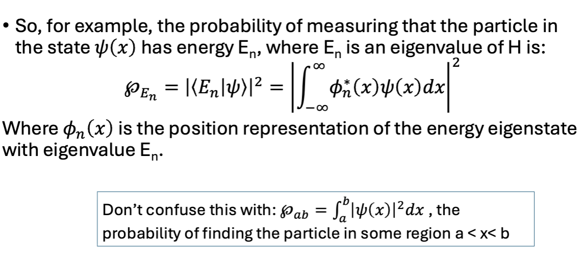
probability of measuring particle in state psi(x) has energy E_n VS. probability of finding particle in some region a<x<b

dirac vs matrix vs wave func: states

dirac vs matrix vs wave func: energy eigenval eqn

dirac vs matrix vs wave func: probability density

dirac vs matrix vs wave func: normalization

dirac vs matrix vs wave func: operators

dirac vs matrix vs wave func: inner products

dirac vs matrix vs wave func: probability of being in a state

dirac vs matrix vs wave func: expectation value

when is inf square well a good approximation

if energy of particle is much smaller than barrier height (ex: e- in nanowire)

The infinite square well is a good approximation when a particle is confined within a rigid, impenetrable barrier with perfectly reflecting walls, allowing for discrete energy levels. This model is useful for analyzing systems where the potential energy outside the well is significantly larger than that within.

wave vector

parameter k that comes from solving inf sq well inside the box

associated with the momentum of a particle according to the de Broglie hypothesis, given by the relation ext{k} = \frac{2\pi}{\lambda} , where \lambda is the wavelength.

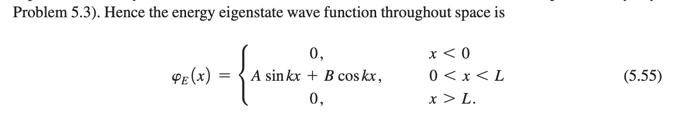
inf sq well wave function

quantization condition

The quantization condition refers to the requirement that the allowed wave functions of a particle in a confining potential must satisfy specific boundary conditions, leading to discrete energy levels.

This occurs in systems like the infinite square well, where only certain wavelengths and frequencies are permitted.

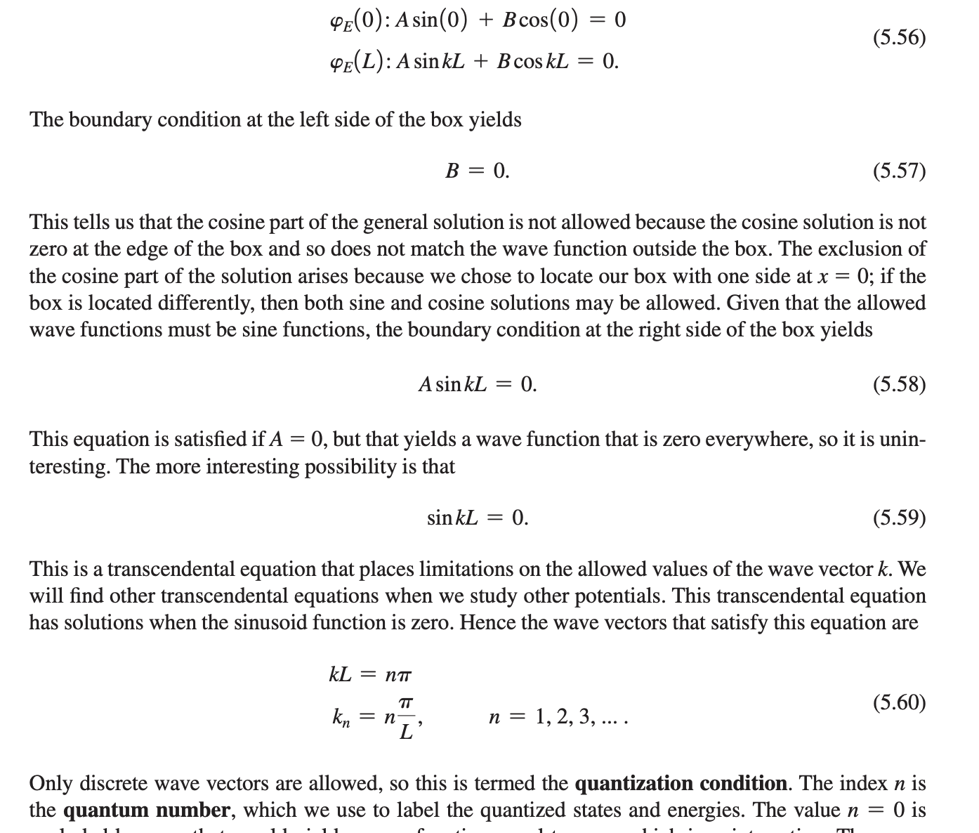
how do we derive n? why must n>0

To derive the quantum number n for a particle in a box, we apply the boundary conditions to the wave function, leading to discrete solutions. The condition n>0 ensures that we only consider physically meaningful states, corresponding to standing wave patterns.

• n from soln to A\sin\left(kL\right)=0

• k_{n}=n\frac{\pi}{L} → if n=0 then wave function = 0 (uninteresting) , exclude negative values bc they yield same states as corresponding positive n values

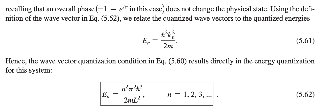
  • overall phase -1=e^iπ doesn’t change physical state

energy quantization of inf sq well

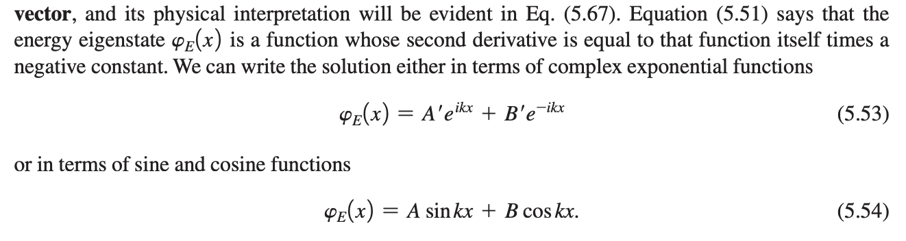
how to determine constants for wave function for inf sq well: \phi\left(x\right)=A\sin kx+B\cos kx

1. use boundary conditions (wave func to 0 at boundary of box)

2. if boundary conditions don’t solve then normalize by integrating and setting =1: 1=\int_{-\infty}^{\infty}\!\phi_{n}^{\ast}\,\left(x\right)\phi_{n}\left(x\right)dx=\int_{-\infty}^{\infty}\!\left\vert\phi_{n}\left(x\right)\right\vert^2\,dx

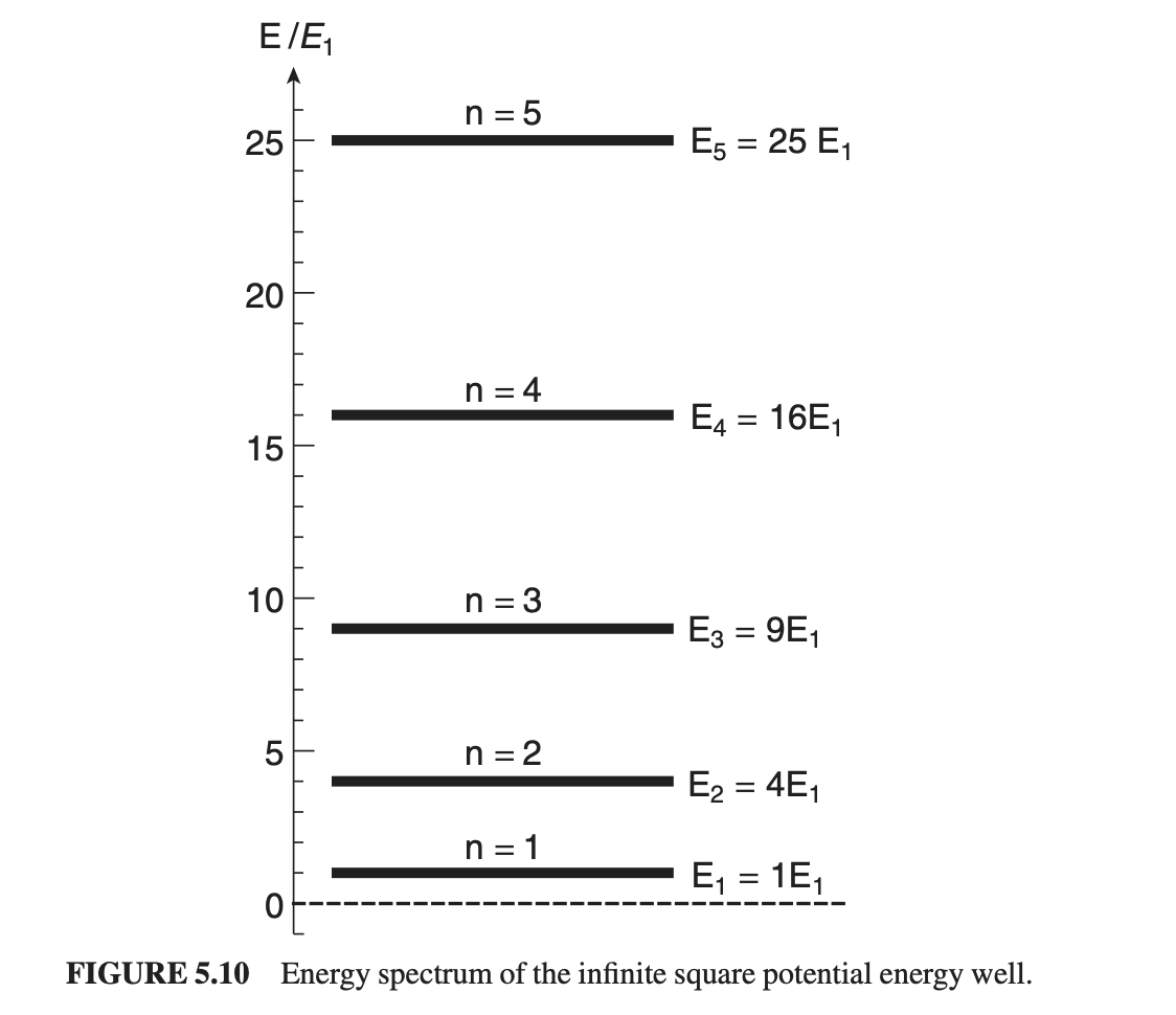
energy spectrum of inf sq well

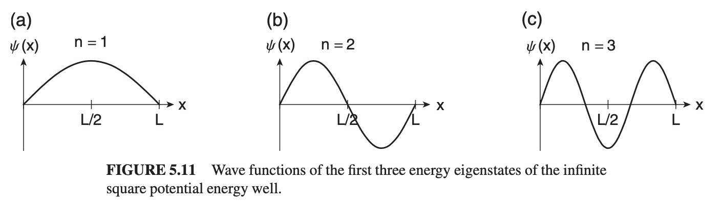
wave functions of first three energy eigenstates of inf sq well

like standing wave with quantized energy levels

wave particle duality

The concept that every particle or quantum entity can be described as either a particle or a wave. This phenomenon illustrates the dual nature of matter in quantum mechanics.

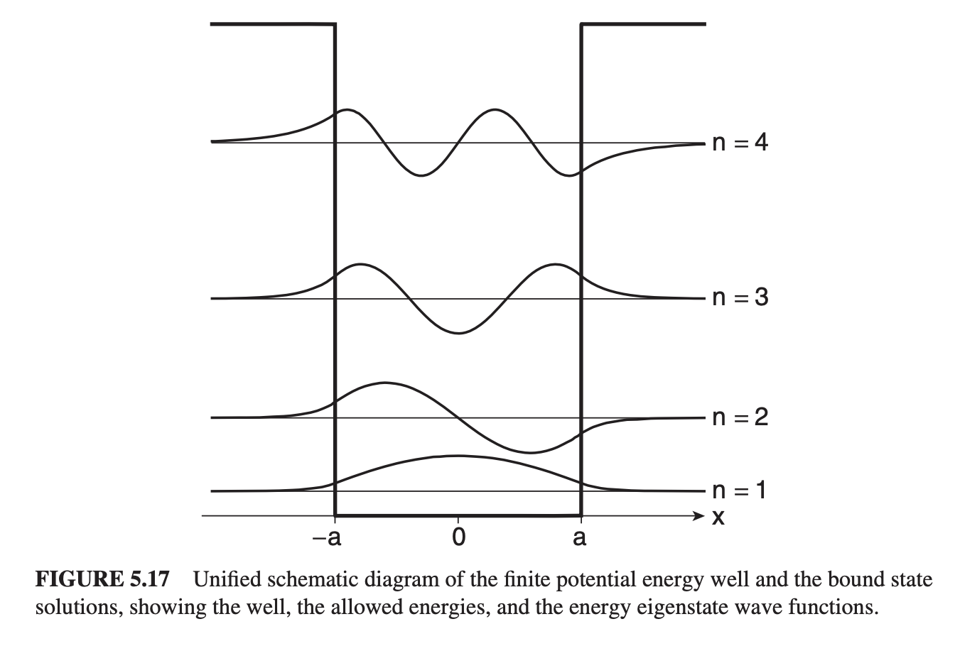
features of waveform solns to infinitq sq well

even-odd parity: n=1,3,5,etc = even wrt center of well; n=2,4,6,etc = odd wrt center of well

nodes: nth soln has (n-1) nodes (not counting edge of well)

general shape is sinusoidal, varying in amplitude and frequency with increasing n.

nodes

locations where there’s 0 probability of finding particle (differs from classical case)

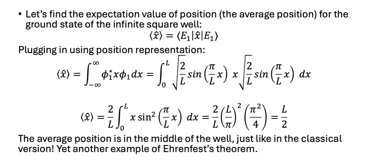
expectation value of position of inf sq well

avg position is in middle of the well (same as classical version ← ehrenfrost thm)

applications of finite square wells

real systems and potential barriers affecting particle confinement.

Examples include quantum dots and traps in atom optics.

ex: electron in thin semiconductor, quantum well semiconductor lasers

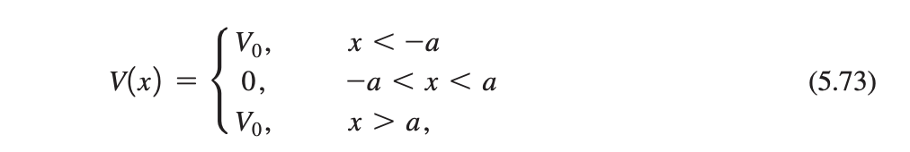
finite square well potential

A potential energy function that describes a particle confined in a region of space with a finite potential barrier, allowing for bound states and tunneling effects.

finite square well potential energy function

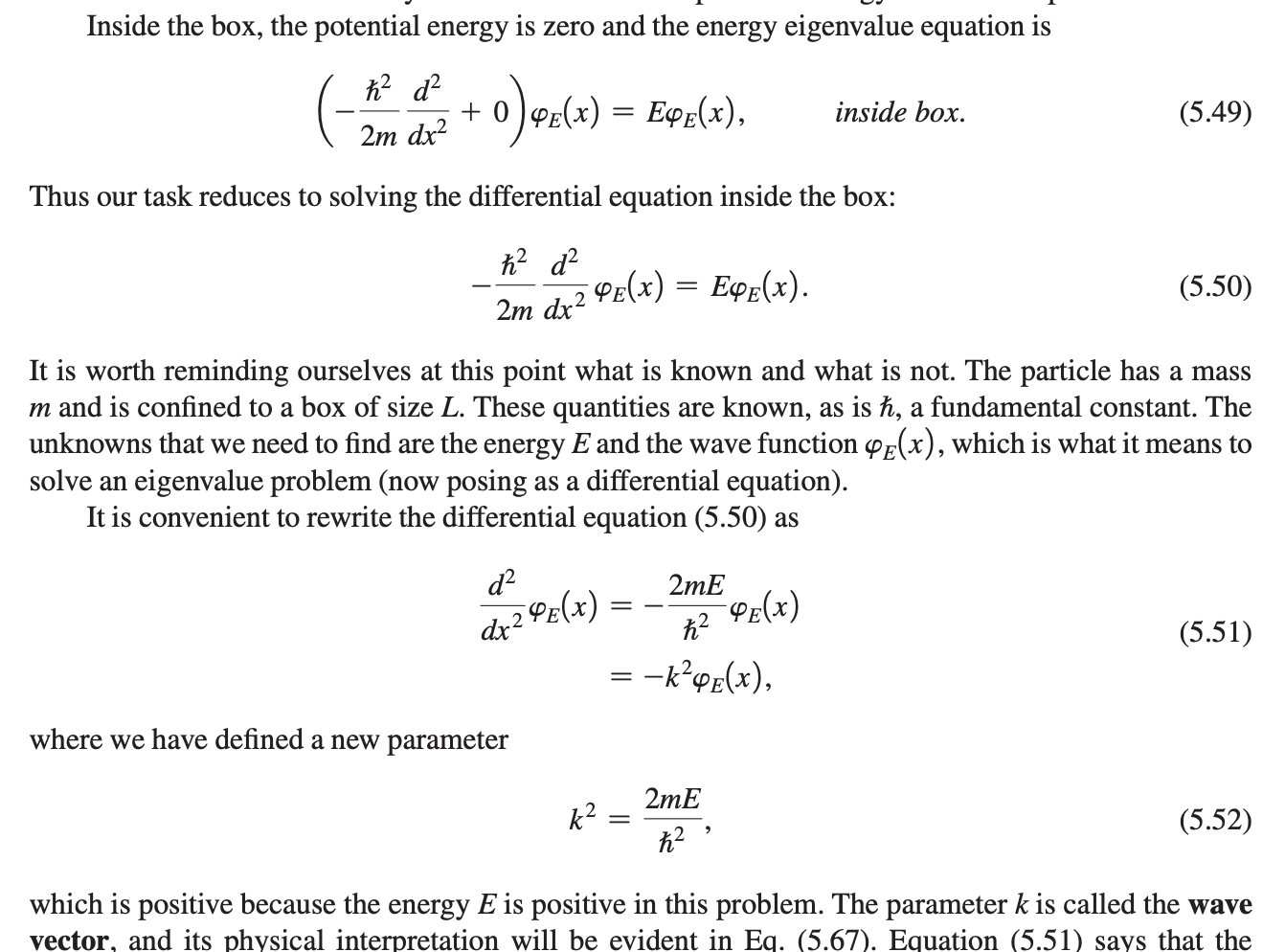
energy eigenvalue equation for finite square well

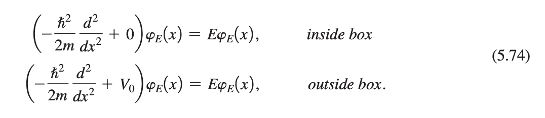
plug in 0 for inside box or V_0 for outside box

constants for inside and outside finite well

inside: wave vector k=\sqrt{\frac{2mE}{\hbar^2}}

outside: constat q=\sqrt{\frac{2m}{\hbar^2}\left(V_0-E\right)} ; derived by solving for \frac{d^2\phi_{E}\left(x\right)}{dx^2}=q^2\phi_{E}\left(x\right)

• q is real and >0 since E<V₀

energy eigenvalue eqn in differential form for finite sq well

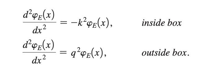
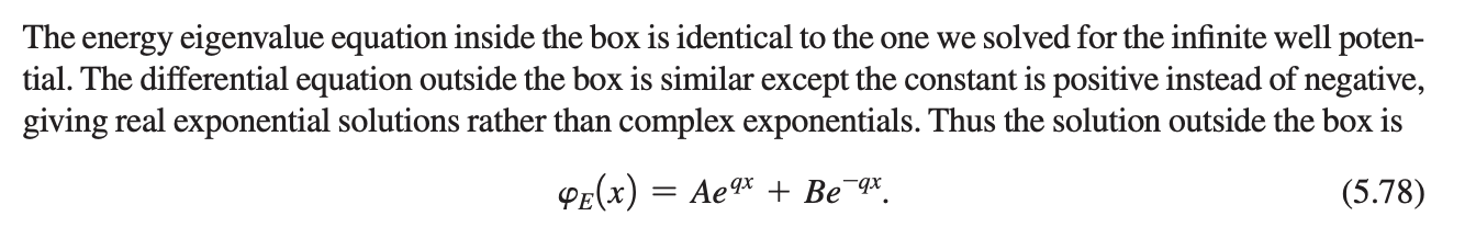
soln for differential eqn inside and outside finite well

inside: same as inside infinte well

outside: constant q is positive so we get REAL exponential solutions rather than complex exponentials

shape of wave function solution in classically forbidden region

exponentially decaying with decay length of 1/q

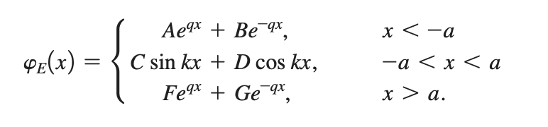
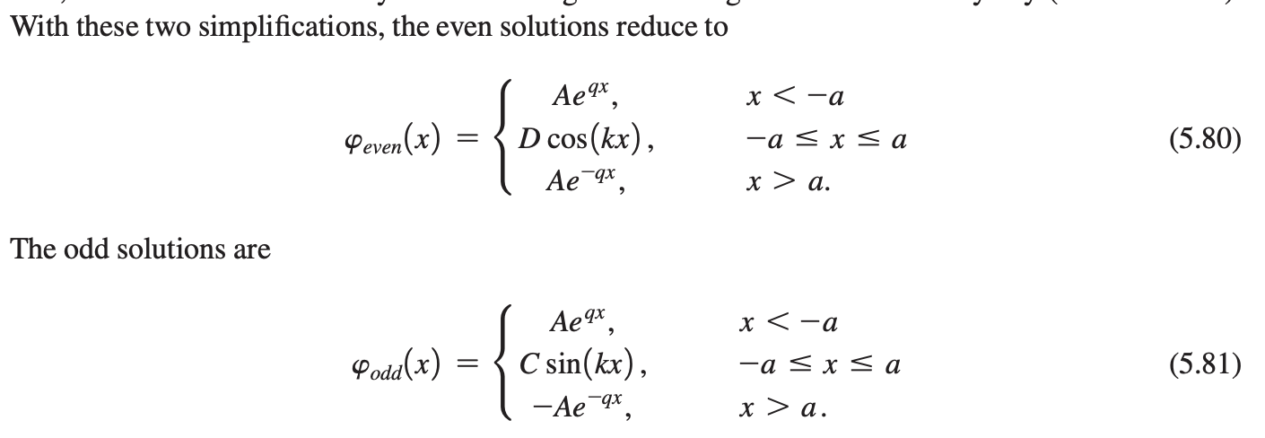
general solution of finite well

boundary conditions for wave function for infinite well

normalization of finite well that differs from infinite well

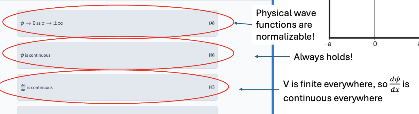
in regions OUTside well, the wave function must be a decaying exponential bc a growing exponential term all the way out to infinity would NOT permit wave function to be normalized → this is a NORMALIZATION CONDITION

boundary conditions for wave function for finite well

in general solution of finite well which constants must be 0 and why

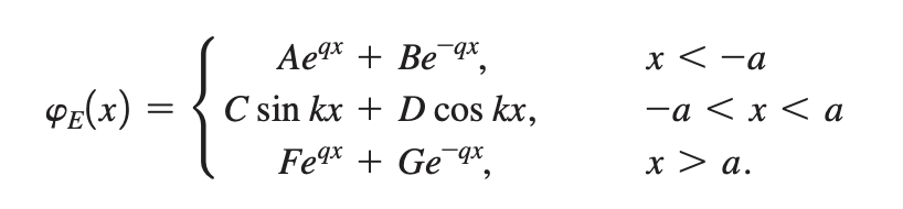
normalization aka boundary condition: in regions OUTside well, the wave function must be a decaying exponential bc a growing exponential term all the way out to infinity would NOT permit wave function to be normalized → this is a NORMALIZATION CONDITION → B = F = 0

since potential energy is SYMMETRIC with respect to origin (V(x) = V(-x)) energy eigenstates will either be symmetric (even) or antisymmetric (odd) → even solutions mean C = 0, odd solutions mean D = 0

transcendental equations

Equations that involve transcendental functions such as sine, cosine, exponential, or logarithmic functions, which cannot be solved algebraically. They often arise in boundary value problems like quantum mechanics and wave functions.

z vs. z₀

dimensionless parameters to simplify transcendental equations

z=ka=\sqrt{\frac{2mEa^2}{\hbar^2}} → z parameterizes energy of the eigenstate

z_0=\sqrt{\frac{2mV_0a^2}{\hbar^2}} → z₀ parameterizes depth of finite well; characterizes the strength of the potential energy well

what is qa equal to

qa=\sqrt{\frac{2m\left(V_0-E\right)a^2}{\hbar^2}}

how to re-express z and z₀ in terms of ka and qa

\left(ka\right)^2+\left(qa\right)^2=z_0^2

\left(qa\right)^2=z_0^2-\left(ka\right)^2=z_0^2-z^2

thus we can rewrite transcendental equations in form:

ka\tan\left(ka\right)=qa\rightarrow z\tan\left(z\right)=\sqrt{z_0^2-z^2}

-ka\cot\left(ka\right)=qa\rightarrow-z\cot\left(z\right)=\sqrt{z_0^2-z^2}

which express relationships between the dimensionless parameters.

in equations above, left side is modified trig function and right side is CIRCLE with radius z₀

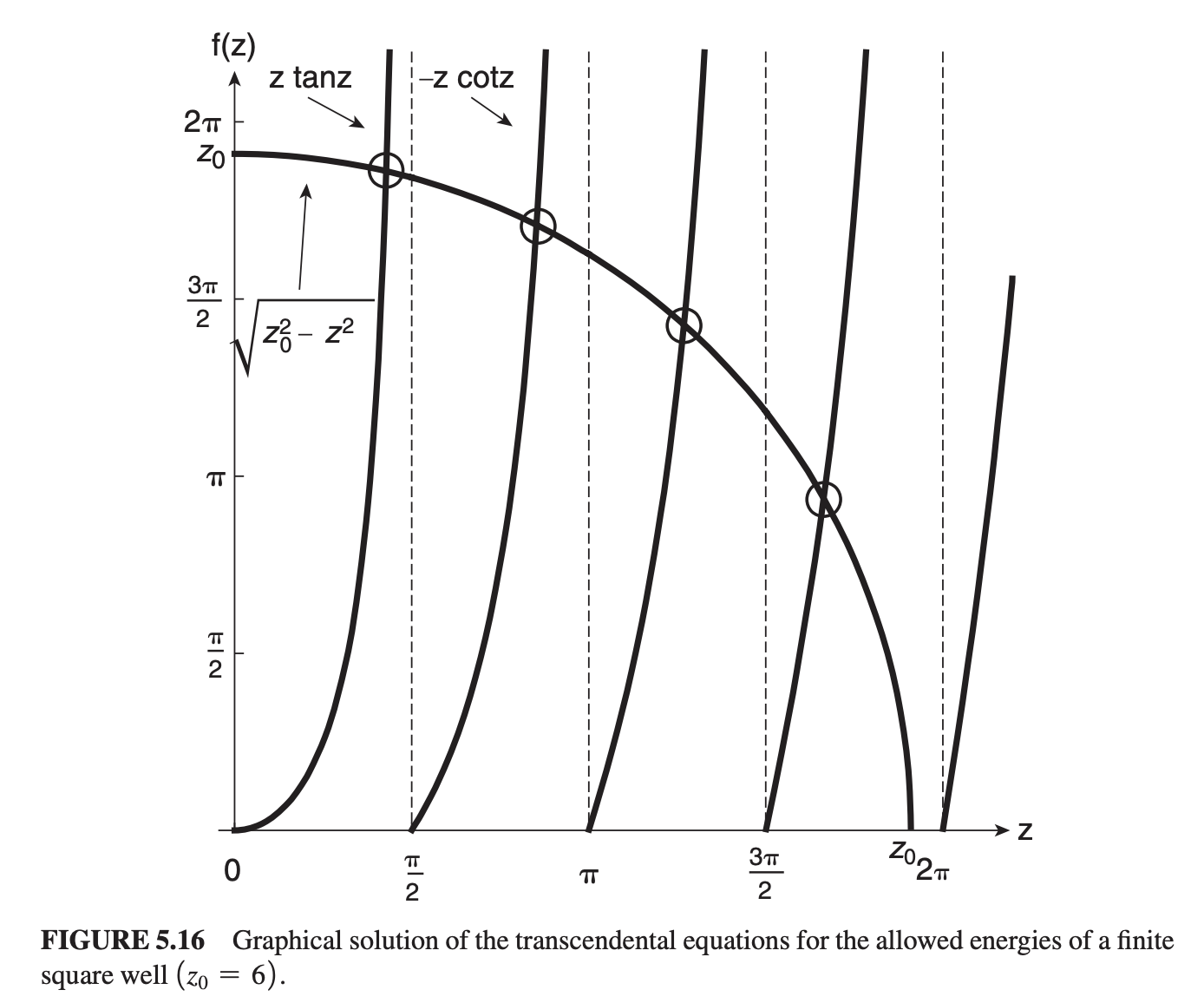
how to plot graphical solution of transcendental equations for allowed energies of finite square well

rewrite transcendental equations in form:

ka\tan\left(ka\right)=qa\rightarrow z\tan\left(z\right)=\sqrt{z_0^2-z^2}

-ka\cot\left(ka\right)=qa\rightarrow-z\cot\left(z\right)=\sqrt{z_0^2-z^2}

left side is modified trig function, right side is circle with radius z₀

if z₀=6 then 4 allowed energies are:

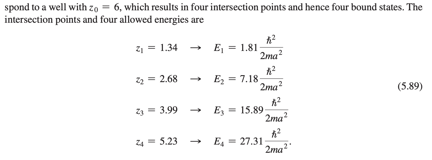
then graph intersection:

barrier penetration

feature of finite well only

when well extends into classically forbidden region

The phenomenon where a quantum particle tunnels through a potential barrier that it classically should not be able to surmount. Barrier penetration occurs due to the wave-like properties of particles in quantum mechanics.

result of barrier penetration

quantum tunneling (example of this is radioactive decay)

how can we get infinite well energy eigenvalues from finite well

take the limit as radius z₀ goes to infinity → allowed values of z become asymptotes of modified trig functions

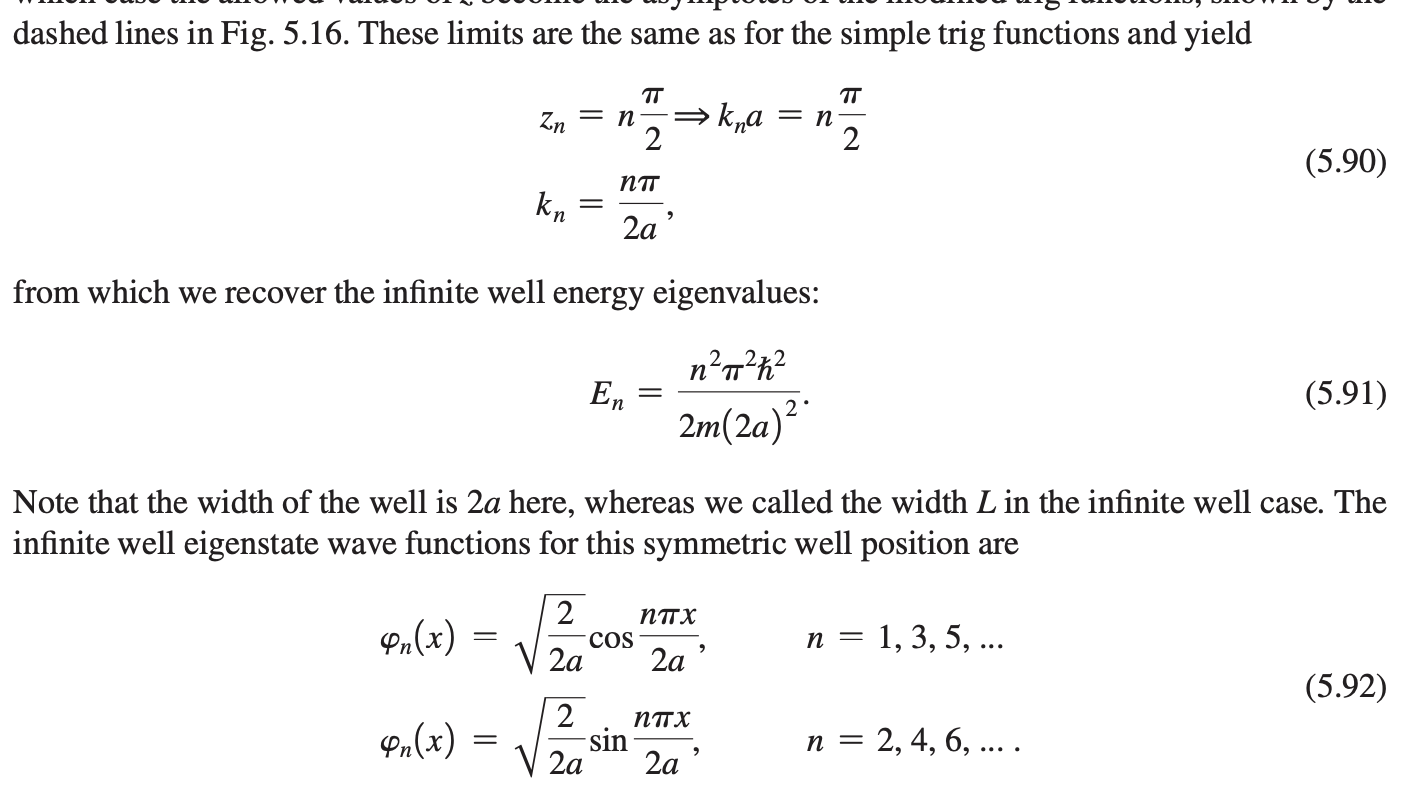
how do we get a deep finite well that resembles an infinite well?

for fixed width a, if V₀ is large, we have a deep well, and z₀ is large