Regression (incl. hypothesis testing), confidence intervals, sum of squares, coefficient of determination

Topic 9

Hypothesis testing - regression

We need to test the estimated equation for the statistical significance of the relationship - if we can show the slope coefficient is different from zero, we can conclude using the regression equation adds to our ability to predict the dependent variable based on the independent variable

Consider y = a + bx + e to be the estimated version of the true regression line y=\alpha+\beta x+\epsilon

We are testing whether \beta parameter is zero or non-zero

so hypothesis test is:

H_0:\beta=0

H_1:\beta\ne0

Confidence intervals - testing significant relationship

Bounds of CI would be given by

b ± t_cvse(b)

t_cv = degrees of freedom t_n-2 distribution for 0.05 sig. level typically

se(b) - standard error

Reject null that \beta =0 if 0 isn’t included in the interval

Or

Find t statistic using

t=\frac{b-\beta}{se\left(b\right)} where beta = 0 and find t critical value and reject H₀ if t > t critical value

\left\vert t\right\vert>\left\vert tcriticalvalue\right\vert

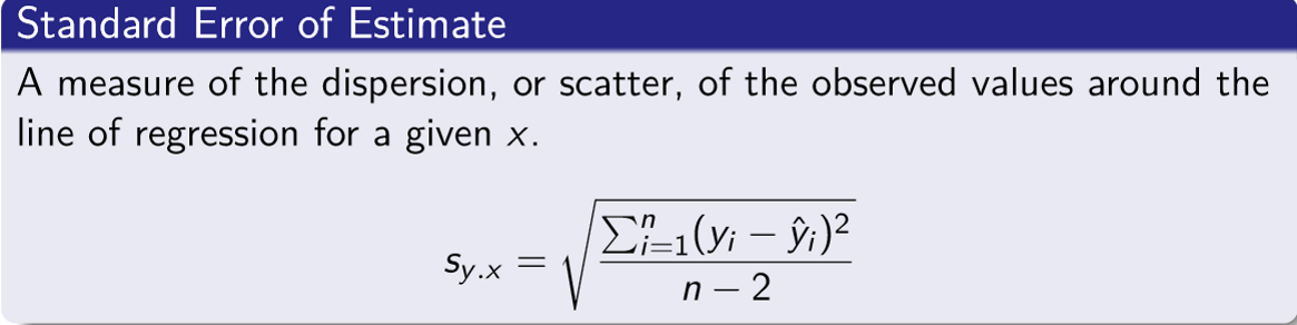
Standard error of estimate

Measures dispersion along the regression line

Formula: image attached

If the standard error estimate is small it indicates the data is relatively close to the regression line and the regression equation can be used to predict y with little error

Coefficient of determination

Most common measure of goodness of fit = R²

Is also inversely correlated to the standard error of estimate

Measures the proportion of the total variation in the dependent variable (y) that is explained by the variation in the independent variable (x)

Ranges from 0 - 1, and closer to 1 = better fit

BUT doesn’t indicated whether relationship is +ve OR -ve

When there is only ONE independent variable the R² is the square of the coefficient of correlation r²

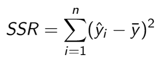
OR can be calculated using R² = SSR/SSTotal

If it is a multivariate model R² would refer to the whole model’s predictive power

Regression Sum of Squares

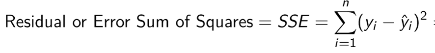
Residual/error sum of squares

Total sum of squares

Sum of regression and error sum of squares

Assumptions underlying linear regression

For each value of x there are corresponding y-values

y-values follow the normal distribution

The means of these normal distributions lie on the regression line

These normal distributions have the same standard deviation

The y values are statistically independent

Relationship between mew ± one standard deviation encompassing 68% of the observations, ± two s.d. encompassing 95% and ± 3 s.d. encompassing almost all of them ALSO applies to predicted values y hat, and standard error of estimate

Confidence interval for the mean of y

Used when the regression equation is used to predict the mean value of y for a given value of x

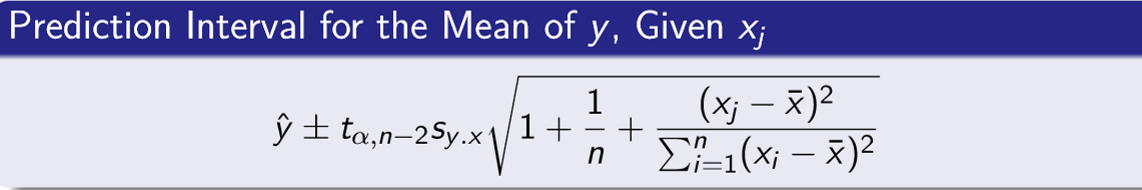
Prediction interval

Used when the regression equation is used to predict an INDIVIDUAL y for a given value of x

Confidence AND prediction intervals

CI:

First substitute the value of x into the y = a +bx to find the midpoint

Then find the critical t value - using n-2 degrees of freedom

Use confidence interval formula and find the range

PI:

Use prediction interval formula

Find t statistic value using n-2 degrees of freedom

PI much larger than CI usually - as intuitively there is a lot of individual variation

Transforming data

Linear regressions assumes the relationship between variables is linear, but what if there is a relationship but it’s not linear

Solution: rescale one or both of the variables so the new relationship IS linear e.g. take the log of the dependent variable y

Other common transformations incl. taking the square root, reciprocal, or square of one of both variables