exam EMF

Economic interpretation first order autocorrelation

Return persistence: when returns are high in month t-1, they tend to be high again in month t. In finance this is consistent with slow adjustment to information

AR(1) model with slope = 0.2 and constant term = 0.01

This month stock return = 0.05, predict next month and month after

R_t = c + phiR_t-1 + u_t

0.01 + 0.2 × 0.05 = 0.02

0.01 + 0.2 × 0.02 = 0.014

Give two approaches to determine how many lags

Start with AR(1) and then see if additional lags matter statistically and economically

AIC = ln(sigma²) + 2k/T

SBIC = ln(sigma²) + k/T ln(T)

SBIC is consistent but inefficient (noisier)

AIC is more stable but inconsistent and tends to pick bigger models

AR(1) model y_t+1 = phi y_{t +} u_t+1 you observe y_t = 0.7, phi = 0.5. Forecast y_t+1 and y_t+2

E[y_t+1] = phi y_t = 0.5×0.7 = 0.35

E[y_t+2] = phi E[y_t+1] = 0.5 x 0.35 = 0.175

Relation to stationarity

if phi < 1, the process is stationarity, shocks die out

if phi > 1, the process is non-stationarity, shocks get amplified

VAR model for interest rate R_f,t and inflation rate I_t

R_f,t = phi₁₁ R_f,t-1 + phi₁₂ I_t-1 + u_1t

I_t = phi₂₂ I_t-1 + u_2t

Work out impulse response function

from t-1 to t shock to inflation of 0.01 and no shock to interest

For time t

I_t = phi₂₂ × 0 + 0.01 = 0.01

R_f,t = phi₁₁ × 0 + phi₁₂ × 0 = 0

For time t+1

I_t+1 = phi₂₂ * I_t = 0.01phi₂₂

R_f,t+1 = phi₁₁ R_f,t + phi₁₂ I_t = 0.01phi₁₂

For time t +2

I_t+2 = phi₂₂ * I_t+1 = 0.01phi²₂₂

R_f,t+2 = phi₁₁ R_f,t+1 + phi₁₂ I_t+1 = 0.01phi₁₂(phi₁₁ + phi₂₂)

Interpret phi₂₂ = 1, what can you say about the impulse function for the inflation rate as we move into the future

In words, moving forward into the future, the shock to the system from time t will never die out.

This does not make much sense economically.

The model for inflation is an AR(1) and the situation at hand introduces a unit root.

If autocovariances of the error term are positive up to lag 12, is the OLS t-statistic correct

No, typically too high. With positive autocorrelation, OLS SE are underestimated, so t-stats took larger values

One way to extend the regression to reduce autocorrelation

Add lagged dependent variables to capture dynamics

Normality test rejected, why is this a problem

In small samples, non-normal errors can make the usual tests unreliable. In large samples less problematic but can still matter with heavy tails

How to test if a period was special

Parameter stability test

Create a dummy for that period and run

yt​ = α + β₁D₁xt ​+ β₂(1 - D₁​)xt + ut

test whether β₁ = β₂

In a regression model the observed y and x are containing a measurement error. Is this a problem for OLS

Measurement error in y

Not for unbiasedness of beta. It mainly adds noise to the dependent variable, larger residual variance, less precise estimates

Measurement error in x

Yes, causes attenuation bias, beta is biased towards zero because x is a noisy version

yt​ = α + βxt + ut

Regression with three different periods. Describe how to extend, formulate the null hypothesis and perform test

yt​ = α + βxt ​+ γ2​D2t ​+ γ3​D3t ​+ δ2​(D2t​⋅xt​) + δ3​(D3t​⋅xt​) + ut

No periods differences means same intercept and slope

H0: γ2 = γ3 = 0 and δ2​ = δ3 = 0

Use F-test of those restrictions

You collect SP500 data (y) and eurostoxx (x)

You run the following regression yt​ = α + βxt ​+ εt

You obtain R2 = 0.784, B = 0.895 and t = 12.3

Interpret the results​

Index levels are typically non-stationary

Regressing one non-stationary series on another produces a spurious regression, high R2

We cannot learn much

If y and x both have a unit root, how to test whether x affects y

Use first differences and then regress

Δyt ​= α + βΔxt ​+ ut​

Here you test whether changes in x affect changes in y

This avoids spurious regression problems

Stock return volatility is persistent. Using daily returns R_t you capture this effect by using an ARCH(1) model

Var(Rt​∣Rt−1​,Rt−2​,…) = α₀​ + α₁R²_t-1

Describe how one could estimate the alpha parameters​

Regress squared return on past squared return

R²_t​ = α₀ ​+ α₁​R²_t-1 ​+ v_t

How to change ARCH(1) model for the variance to incorporate effect of recessions

Var(Rt​∣Rt−1​,Rt−2​,…) = α₀​ + α₁R²_t-1

Let D_t be a recession dummy

Modify variance equation with an interaction

D₁R²_t-1

This allows estimating different slope coefficient for recession vs normal times

Give two ways in which you can test whether the CAPM is the correct model for these stock returns

Test constant term = 0 in the second-step Fama–MacBeth regression

Test slope on beta = average stock market excess return in the second-step regression

You want to estimate a two-factor asset pricing model. First factor is return on stock market index, second factor is change in LT interest rate. How would you estimate the parameters.

First, estimate betas for both factors by running time-series regressions of (stock or portfolio) returns on the market return and the change in the long-term interest rate.

Second, run cross-sectional Fama–MacBeth regressions where you fix the market risk premium equal to the average stock market return (so it is not a free parameter) and estimate the slope on the interest-rate betas. This slope is the risk premium for the second factor.

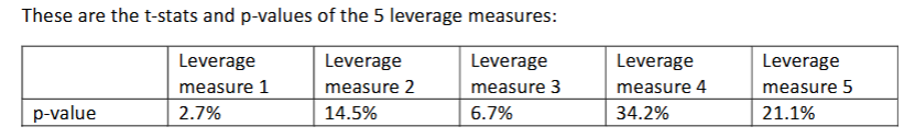
You use 5 ways to measure leverage. For each variable you sort stocks, create a portfolio, and calculate the alpha and pval. Use 95% CI.

You perform a joint test, Gibbons-Ross-Shanken test, whether all 5 alphas equal zero. Pval is 0.5%. What do you conclude and is this the result subject to data mining issues?

Reject the null that all alphas are zero => at least one leverage strategy has a nonzero alpha. No data-mining issues in the test itself because all strategies are tested jointly.

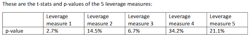
You use 5 ways to measure leverage. For each variable you sort stocks, create a portfolio, and calculate the alpha and pval. Use 95% CI.

Do the Bonferronni adjustment to the pvals. What do you conclude on the existence of a leverage anomaly after doing this adjustment, also in light of the outcome of the test of question a.

Adjusted significance level = 0.05 / 5 = 1%

No individual alpha is significant

Evidence that some leverage anomaly exists, but unclear which measure drives it.

Why is the LASSO coefficient closer to zero compared to OLS?

Because LASSO applies an L1 penalty to large coefficients that shrinks coefficients towards zero

Why is R2 of OLS larger than R2 of LASSO?

OLS maximizes in-sample fit, while LASSO sacrifices some fit to control for variance via the penalty.

Which estimate is better, OLS or LASSO?

OLS is better for inference and in-sample fit

LASSO is better for out-of sample prediction and variable selection

No superior

Use a calendar time portfolio approach for long-horizon event studies, which uses the returns on a portfolio of firms that experienced an event in the past H months.

What is an advantage of this method over standard event study method that uses CARs?

They are robust to event clustering and correspond to a feasible trading strategy

Regression of returns on a calendar time portfolio of IPO firms

Where MKT is the market excess return, and SMB is the size factor return Small minus Big and VMG is value factor return Value minus Growth

Indicate what type of firms have an IPO

Positive SMB and negative VMG loadings, small growth firms

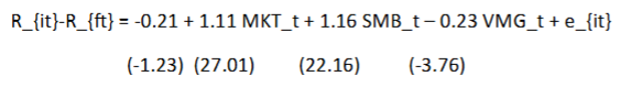
Regression of returns on a calendar time portfolio of IPO firms

Where MKT is the market excess return, and SMB is the size factor return Small minus Big and VMG is value factor return Value minus Growth

What can you conclude about the long-run performance of IPO firms

Alpha is negative but not statistically significant, no evidence of long-run underperformance