Intermediate Macroeconomics Semester 1 key terms

Keynes 3 conjectures:

Keynes conjectures

• DY = main consumption determinant

  • positive proportional relationship

• MPC = 𝜕𝐶/𝜕𝑌 ≈ Δ𝐶/Δ𝑌

  • somewhere between 0-1

• APC: ratio of C:Y

  • Y increases, APC decreases

  • APC = C / Y

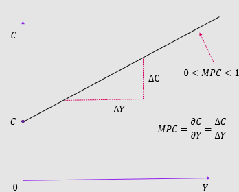
Keynesian consumption function:

Keynesian-consumption-function: C = 𝐶2+𝑀𝑃𝐶×𝑌

C2 = 𝐶 ̅ = autonomous consumption ; intercept

• 𝐶 ̅ = intercept, MPC = slope, Y = exogenous variable, C = endogenous variable

• DY = Main determinant, 0 < MPC < 1

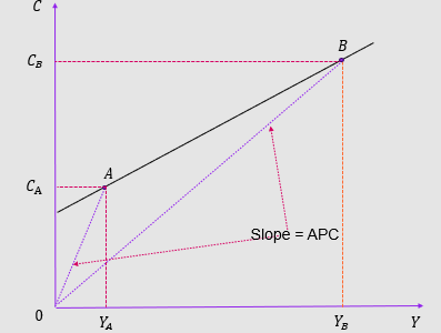
APC and the Keynesian Consumption Function:

Average Propensity to Consume calculation

1. C = 𝐶 ̅ + MPC x Y

2. APC = C / Y

3. APC = 𝐶 ̅ / Y + (MPC x Y) / Y

4. APC = C / Y + MPC

   1. Y cancels out

Therefore, increased Y reduces APC

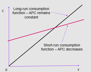
Analysis of the Keynesian consumption function and predictions: 

• initial positive empirical research

• Predicted Y > C in terms of growth —> did not come true

  • predicting fall in C —> increase in I

  • Y grew —> APC constant —> similar growth of C

  • C/Y stability in L-T time series data

• Outcomes:

  • S-T constant APC

23rd of September 2022 Chancellor Kwasi Kwarteng announced a cut in the basic rate of income tax from 20 to 19 per cent. The change is to take effect from April 2023. Explain when and how this tax cut would impact consumer spending according to the Keynesian consumption function.

1. cut in basic tax rate

2. increase in DY —> increase in consumption (move along 𝐶 ̅ curve - graphical)

3. dependent on MPC (slope)

   1. Δ𝐶 = MPC x Δ𝑌, if Y increase and MPC is constant (S-T), C increases

4. Change in consumer spending in April 2023, changing DY

Q) What do you think the authors mean by saying that the MPC depends on the details of recipients?

• details of recipients - consumer behaviour, level of savings, prior income, income from assets, state of the economy

“the aggregate response to a transitory income shock should depend on the details of recipients” Caroll et al. (2017, QE)

Intertemporal budget constraint:

Intertemporal budget constraint

• Assumes consumer is forward-looking; maximise satisfaction for present and future

• Definition: A measure of the total resources available for present and future consumption

• PV of C= PV of Y

Basic model and components of the Intertemporal budget constraint:

Basic model:

• two time periods = t and t+1

• Real Income = Yt and Yt+1

• Real Consumption Expenditure = Ct and Ct+1

• Real savings = St

• Real IR on bonds = r, same for lending and borrowing

💡

• Real budget constraint at time t = Ct + St = Yt

• Real budget constraint at time t+1 = Ct+1 = Yt+1 + (1+r)St </aside>

• Savings carried over to t+1

• If St > 0 = saving

• If St < 0 = borrowing

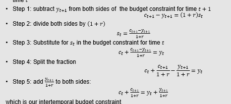
Deriving intertemporal budget constraint:

Calc) We want to derive an intertemporal budget constraint. We need to combine the budget constraint for period t with that for period t+1. We do it by deriving St from the budget constraint for time t+1 and plugging it into the budget constraint at time t.

Intertemporal budget constraint: Ct + Ct+t / 1+r = Yt + Yt+1 / 1+r

• dependent on r prior to t+1

• dividing by 1+r —> finding present value

  • PV x (1+r) = FV

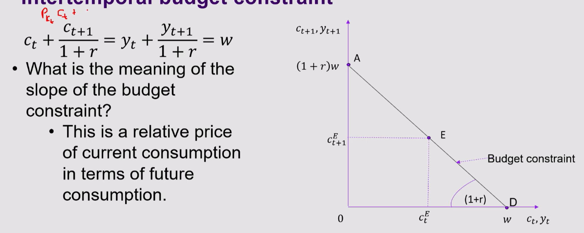
Inter-temporal budget constraint:

The slope of the budget constraint is the relative price of current consumption in terms of future consumption.

• a change in current or future income shifts the IBC.

• The IBC rotates when the real IR changes

  • increase in IR —> slope is steeper

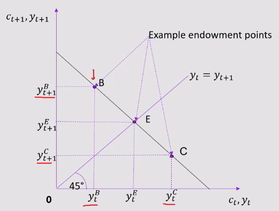
Endowment point: 

Endowment point determines exogenous income at time t and t+1

Assumptions of consumer preferences:

• shown with indifference curves

Assumptions:

• more is better

• preference for diversity

• Consumption today and tomorrow are normal goods

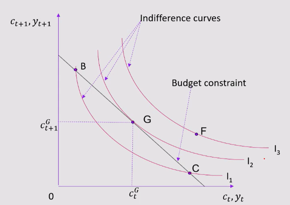
Optimal point on the Budget Constraint:

The optimal point on the slope of the budget constraint is equal to the slope of the indifference curve

• (1+r) = MRSct, ct+1

• a rate at which consumer is willing to give up future consumption to get a unit of current = market prevailing rate

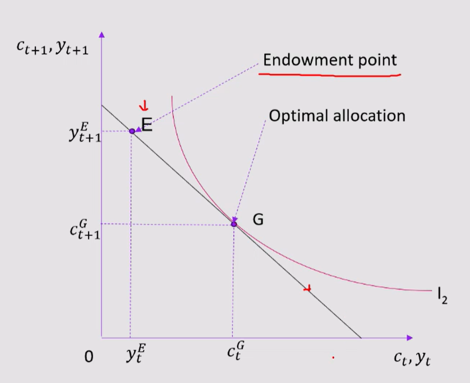
Optimal choice analysis: 

• At point B the consumer is a borrower, and at the red point is where a lender would be placed

• 0YET = income at t

• OCGT = consumption at time t, so income < consumption, hence borrowing due to diff

• OYET+1 = income at t+1

• OCGT+1 = consumption at t+1

• together —> borrowings + interest / savings + interest —> borrower / lender

Application Q of intertemporal budget constraint and indifference curves (IMPORTANT)

Application:

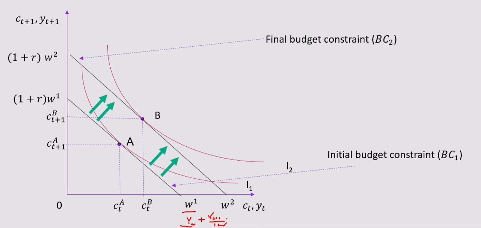
The $1.9 trillion economic stimulus signed into law by Biden on March 11, 2021, included among others $1,400 direct payments to individuals.

Q1) In a two-period model, show on a graph the impact of such transfer on consumption

• assume instant transfer + assume future distribution

• Horizontal axis = present consumption or income (Ct, Yt)

• Vertical axis = future consumption or income (Ct+1, Yt+1)

• Everything on x-axis is t, and everything on Y axis is t+1

  • wages are (1+r) as slope of constraint is dependent on IR

• BC1 is initial budget constraint, based on initial wage / income w1

• BC2 is final budget constraint, after increased to w2 (shifts out)

• shift out indicates higher lifetime income w2 > w1 (+$1,400 direct payment)

• I1, original indifference curve, optimal point = A (centre, bowed origin)

• I2, new indifference curve, optimal point = B

• Moving A —> B shows consumer achieving higher level of utility (I2 > I1)

• A = optimal consumption when wage = w1 (Ct A, Ct+1A)

• B = new optimal consumption when wage rises to w2 (Ct B, Ct+1B)

• Therefore, pure income effect of higher wages —> higher ct and higher utility

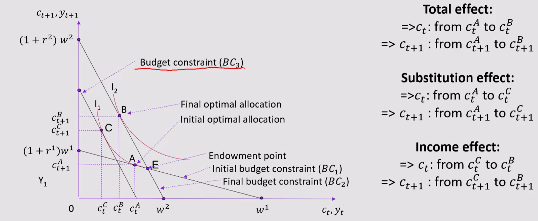
Question 2) BOE raises IR by 0.25 pp to 5.25%. In a two-period model show the impact of such change on lenders, comment and how does this compare to Keynesian consumption function?

Hint - lender; where is optimal point with respect to endowment point

Hint - budget constraint after change will have to go through endowment point

Hint - slope of BC

Phase 1) Solution

• Horizontal axis = present consumption or income (Ct, Yt)

• Vertical axis = future consumption or income (Ct+1, Yt+1)

• Everything on x-axis is t, and everything on Y axis is t+1

  • wages are (1+r) as slope of constraint is dependent on IR

• plot endowment point and BC go through

• BC1 is initial budget constraint, based on IR change at w1

• BC2 is final budget constraint, after IR causes decreases to w2 (shifts in, gets stepper)

Phase 2) Lender 1

Increase in IR implies stepper ITBC

• Optimal allocation moves from A to B

  • A is initial allocation —> B is final allocation

  • A (Cta, Ct+1A) —> B (CtB, Ct+1B)

• Initial indifference curve of I1 at point A —> I2 at point B

• Current consumption has decrease from CtA —> CtB

  • encourages savings —> increase future consumption (Ct+1A —> Ct+1B) as future income is higher

Phase 3 - Lender 2

budget constraint C, parallel so change is already incorporated (BC3)

• tangent to initial indifference curve I1 (on same curve as A)

• Same level of utility as point A due to same indiff curve

• A —> C, increasing IR decreasing current consumption and reduce future consumption (substitution effect)

• C —> A, outward shift in BC (income effect) as income is higher due to savings generation from higher IR, mainly for savers.

Therefore 

• Substitution effect < Income effect, empirically supported, in this case

• Interest rate increase: lender

  • C+ —> SE (-), IE (+) —> SE + IE = ?

  • Ct+1 —> SE (+), IE (+) —> SE + IE > 0

(vice versa if IR decreases)

• Interest increase: borrower

  • Ct —> SE(-), IE (-) —> SE + IE < 0

  • Ct+1 —> SE (+) , IE (-) —> SE + IE = ?

(vice versa if IR decreases)

Life-Cycle Hypothesis assumptions and model:

Life-Cycle Hypothesis

• Consumption depends on lifetime income, and people try to achieve a smooth consumption pattern; varies systematically over phases + savings = goal achieved

  • W = initial wealth

  • Y = annual income until retirement (constant)

  • R = number of years until retirement

  • T = lifetime (yrs)

• Assumptions:

  • Zero real IR

  • Smoothing = optimal

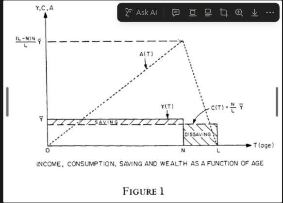
Life Cycle hypothesis (Modigliani 1986, AER p.300)

Y- annual income; A – wealth; N – number of years one works; L – number of years one lives; C – consumption

SR policy implications and criticism of LCH:

SR policy implications

• Monetary Mechanism

• Transitory Income Tax changes

Criticism: (saving behaviour of elderly)

• uncertainty

• bequest motive

Permanent Income Hypothesis

Permanent Income Hypothesis

Y = Y^P + Y^T

Y = current income

Y^P = permanent income; average income expected in future

Y^T = transitory income; temporary deviations from average income

• Consumers use savings and borrowings to smooth consumption in response to transitory changes in income

PIH CF: C = aY^P

• a = fraction of Y^P consumed per year

• Implies: APC = C/Y = aY^P/Y

  • High Y households have on average a higher transitory income than low Y

    • APC = lower in High Y houses.

  • LR income variation due to variation in Y^P, implying stable APC

Application of LCH, PIH:

Assume you are a 50-year-old who expects to work for additional 25 years and then enjoy 15 years of retirement. If you behave according to the life-cycle/permanent income hypothesis, how would your current consumption change if:

• You win £1,000,000 in the lottery this year.

You win in the lottery £10,000 paid each year by the end of your life

• LCH:

  • Annual income until retirement is £10,000 greater

  • Initial wealth only marginally changes by £10,000

  • APC should decrease and thus be lower than lower income households

  • Transitory Income Tax Changes due to injection of wealth (tax on winnings)

  • Consumption would increase but would follow smooth pattern

  • uncertainty - large portion may be saved, APC may decrease

• PIH:

  • Higher transitory income

  • Injection of lottery winnings is transitory deviation of income

  • in the LR, APC will be stable

Random-walk Hypothesis (Robert Hall, 1978)

Random-walk Hypothesis (Robert Hall, 1978)

• based on LCH, PIH, adds assumption of rational expectations

  • People use all info to forecast future variables like income

• Random walk: changes in consumption should be unpredictable

• An anticipated change in Y or w has already been factored into expected Y^P

  • thus consumption is constant

• Only unanticipated changes in income or wealth that alter expected Y^P will change C </aside>

• No response of anticipated Y change due to soothing

• MPC of transitory shock should be small, permanent = closer to 1

“Consumption reaction to permanent shocks is much higher than that to transitory shocks”

• Jappelli and Pistaferri (2010, Annual Review of Economics)

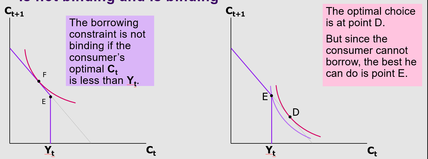
Borrowing constraint (binding vs non-binding)

• Constraint is not binding if OPT Ct < Yt, point F

• Optimal choice is D, constraint is binding, best point is E (Cannot borrow)

• Budget constraints can shift too

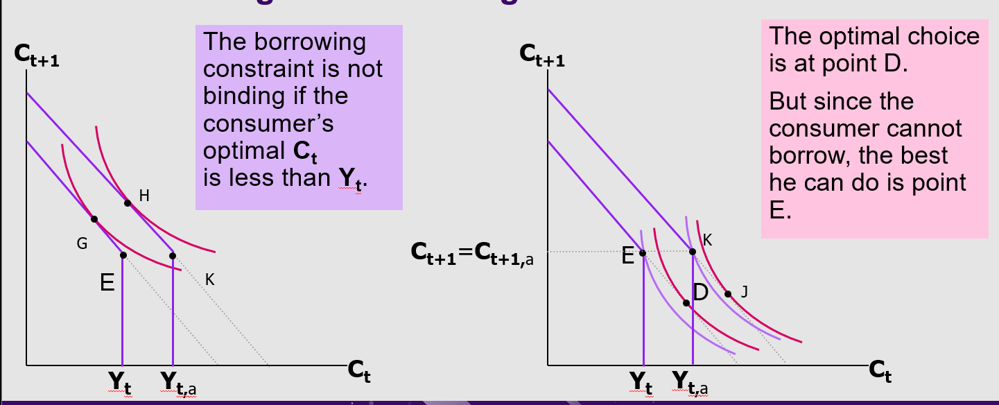
Consumer optimisation when BC is not binding vs binding:

• Constraint is not binding if OPT Ct < Yt, point F

• Optimal choice is D, constraint is binding, best point is E (Cannot borrow)

• Budget constraints can shift too

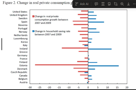
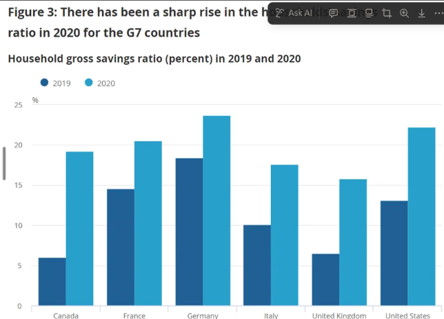
Precautionary savings: (Mody et al, 20102, IMF WP)

• Mody et al. (2012) show that there was a significant increase in savings and a drop in consumption - and that at least 40% of savings were due to precautionary motives. • For example, Carrol and Samwick (1998) indicate that roughly 40-45% of savings is due to the precautionary savings

Cobb Douglas Production Function:

Y=𝐴𝐾^𝛼 𝐿^(1−𝛼)

• 0 < 𝛼 < 1 denotes output elasticity of capital

• A = total factor productivity

• Y = output

• K = capital input

• L = Labour input

Marginal product of capital and conclusions:

Marginal-product-of-capital: MPK = 𝜕Y / 𝜕K

MPK = 𝜕Y / 𝜕K = 𝛼𝐴𝐾^(𝛼-1) 𝐿^(1−𝛼) > 0

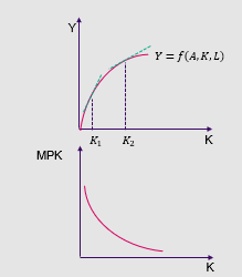
• Law of diminishing returns: find 𝜕MPK / 𝜕K

• An increase in capital decreases marginal product of capital

• An increase in capital increases output at a diminishing rate

Neoclassical model of investment

Neoclassical model of investment

• Investment depends on MPK, IR and tax rules

  • Assumptions:

    • Production firms rent the capital they use to produce G&S

    • Rental firms own capital, rent to production firms

    • Investment = rental firms spending on new capital

Profit of a production firm:

• Profit of a production firm:

  Π=𝑃𝑌−𝑅𝐾−𝑤𝐿

• Π = profit

• P = price

• Y = output

• R = rental rate of capital

• K = capital stock

Calculate Profit Max for a firm under Investment topic:

First order condition:

• 𝜕Π / 𝜕K ; to max Π, firms will increase capital up to where MPK = R / P

1. FOC : 𝜕Π / 𝜕K

2. Profit : Π = 𝑃𝐴𝐾^(𝛼-1) 𝐿^(1−𝛼)−𝑅𝐾−𝑤𝐿

3. FOC w.r K : 𝜕Π / 𝜕K = 𝛼PAK^(𝛼-1)𝐿^(1−𝛼) - R = 0

   1. 𝛼-1 comes down and -1 to leave 𝛼, rest is the same

   2. L^(1-𝛼) = constant (because respect to K)

   3. RK —> K drops out respectfully

   4. wL = constant)

4. Rearrange: 𝛼PAK^(𝛼-1)𝐿^(1−𝛼) = R

5. Rearrange (/ both sides by P): R/P = 𝛼PAK^(𝛼-1)𝐿^(1−𝛼); PROFIT MAX

Profit max: R/P = 𝛼PAK^(𝛼-1)𝐿^(1−𝛼)

EQ R/P would increase if:

• K decreases (e.g. earthquake / war)

• L increases (e.g. pop growth / immigration)

• A increases (tech improvement / deregulation)

Rental firm’s investment decisions and components of capital cost:

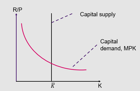
• Rental firms invest in new capital when benefit > cost

• Benefit (per unit capital) : R/P (income from renting capital)

Components of capital costs:

Interest cost: i x Pk

• Pk = nominal price of capital </aside>

Depreciation cost: δ x Pk

• δ = rate of depreciation </aside>

Capital loss: - ΔPK

• capital gain ΔPK > 0, reduces cost of K </aside>

Nominal-cost-of-capital: iPk + δPk - ΔPK = Pk + (i + δ - ΔPK / Pk )

Rental firm’s profit rate:

Rental firm’s profit rate:

• A firm’s net investment depends on its profit rate

Profit-rate = R / P - Pk / P (r + δ ) = MPK - Pk / P (r+δ)

• If PR > 0, increasing K = profitable

• If PR < 0, firm increases profits by reducing capital stock (not replacing during depreciation)

Taxes and Investment + Corporate income tax: 

Taxes and Investment:

Investment tax credit:

• ITC reduces firm taxes by a certain amount for each dollar it spends on capital

• ITC reduces Pk —> increases Profit rate and investment incentive

Corporate income tax: 

• Our definition= rental price - cost of capital

  • Dep cost measured using current capital price —> Corp income tax does not affect investment

• if Pk rises overtime, legal definition (using historical price of capital) understates true cost and overstates profit —> corporate tax discourages investment

Net and gross investment:

net investment = ΔK=In [MPK−(P_K/P)(r+δ)]

gross investment = ΔK+δK=In [MPK−(P_K/P)(r+δ)]+δK

• Ln {} is a function that shows how net investment responds to an incentive to invest

• Total spending on business fixed investment = net investment + replacement of depreciated K

Two phases of investment function:

Investment function

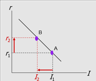
• gross investment = ΔK+δK=In [MPK−(P_K/P)(r+δ)]+δK

Phase 1:

• An increase in r:

  • raises capital costs, reduces profit rate, reduces investment

Phase 2:

An increase in MPK or decrease in Pk/P:

• increase profit rate, increases investment at any given r

• shifts I curve to the right

Tobin’s q equation and explanation

q = Market-value-of-installed-capital / replacement-cost-of-installed-capital

• numerator: stock market value of economy capital stock

• denominator: actual cost to replace goods that were purchased when stock was issued

• if q > 1, firms buy more capital to raise their market value

• if q < 1, firms do not replace capital due to depreciation

• Investment is likely to rise if productivity or output prices rise and r falls —> Increased MV

  • also encouraged by fall in capital cost

• Main feature: Current Investment will be influenced by future values of these variables

A wave of pessimism about future capital profitability would cause:

1. stock prices fall due to uncertainty

2. Tobin’s q would fall as capital costs are foreseen to rise

3. shift the investment function down due to reduced willingness to invest / higher risk

4. Negatively shock AD (considering Inv is falling)

A fall in stock prices would: 

1. reduce household wealth

2. shift consumption function down (due to reduced level of income, increased MPS)

3. Negatively shock AD (considering C is falling)

A fall in stock prices may impact expectations of what and how?

1. A fall in stock prices might reflect negatively about technological progress and LR EG

   1. AS and FEQ will be expanding slower than expected, thus expectations may fall

Residential investment and how its determined:

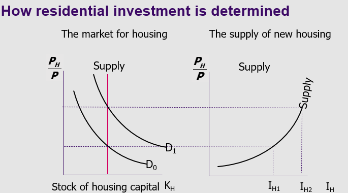
• the flow of new residential investment, IH, depends on relative price of housing

  • PH / P

    • determined by D&S for existing households

  • Stock housing capital KH

Flow of residential investment IH is x axis for 2nd graph

• An increase in supply of KH shifts out demand curve for housing from D0 to D1 with constant supply, in line with a movement along the supply curve for new housing as residential investment increases

  • Therefore, residential investment is determined by an increase in demand for housing, encouraging an increase in supply of new housing to satisfy the demand

Inventory investment and recessions:

1% GDP, but during a recession, 50%+ the fall in spending is due to a fall in inventory investment

4 motives for holding inventories:

• Production smoothing:

  • Sales fluctuate, but steady production is cheaper

  • When s < p, Inventories rise

  • when s > p, inventories fall (as a given)

• Inventories as FoP:

  • Allow for efficient operation

    • samples for retail sales purposes

    • Spare parts when machines fail

• Stock-out avoidance:

  • to prevent lost sales in the event of excess demand

• Work-in-progress:

  • Goods not yet completed are counted as part of inventory

Origin of Keynesian Economics:

• developed around Great Depression

• US - rising UN and falling real GNP vs Great Britain - High UN in 1920s and 30s

• Keynes: Problem = LACK OF AD

  • EQ Y = AD

    • Assume closed:

      • Agg PL fixed

      • Real variables

Keynes Cross Equilibriums:

1. Output = AD

   Y = C+I+G

2. Output = NI

   C+I+G = Y = C+S+T —> S + T = I + G ; C-cancels-out

3. Output = National Product

C + I^r + G = Y = C + I + G ; I^r = I

Algebra for Keynes EQ + Balanced budget multiplier with MGC and MT: 

Y = C + I + G

C = a + bYd = a + b(Y-T) ; T = lump-sum taxes

Y = a + bY - bT + I + G

Multiplier for GC = ∆𝑌/∆𝐺 = 1 / 1-b

Multiplier for taxes = ∆𝑌/∆T = - b / 1-b

Balanced-budget multiplier:

∆𝑌/∆𝐺 + ∆𝑌/∆T = 1 / 1-b + (- b/1-b) = 1 / 1-b - b / 1-b = (1-b)/(1-b) = 1

Factors affecting slope of IS curve: 

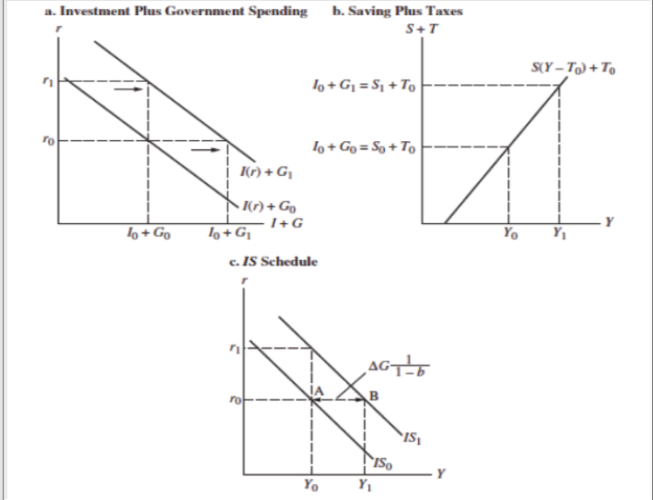
1. Slope of Investment schedule

I - interest elasticity of investment demand is low

I’ – interest elasticity of investment demand is high

• IS = steep when I and vice versa

• Extreme = when I = 0, Investment and IS are vertical

2. Slope of Savings Function (b)

• IS steeper when MPS is higher e.g. S(Y) MPS 0.8

• IS flatter when MPS lower e.g. S(Y) MPS 0.3

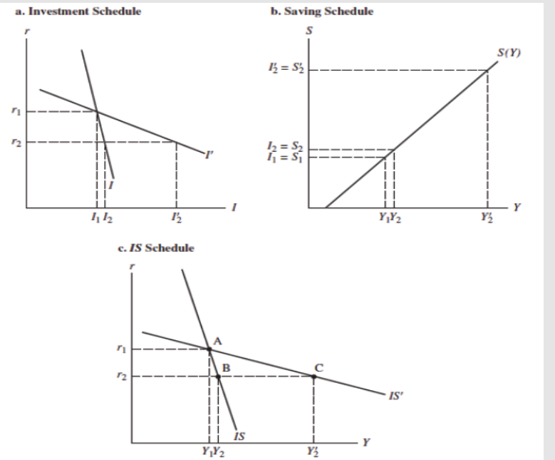
Shifts in IS Schedule:

• changes in G

  • Increase G —> Increased AD —> IS shifts right (vice versa)

• changes in Autonomous I

  • Confidence or expected Profitability rises —> Autonomous I increases —> IS shifts right (vice versa)

• change in taxes

  • Decreased T —> higher DY and C —> IS shifts right (vice versa)

Savings and investment function for IS Schedule:

I + G = S + T

Savings function

S = -a + (1-b)Yd = -a + (1-b)(Y-T)

Investment function:

I = 𝐼bar - i1r

where i1 > 0:

𝐼bar = i1r + G = -a + (1-b)(Y-T) + T

Rearrange:

Y = 1 / 1-b (a + Ibar + G - bT - i1r)

Ibar = I ̅

Financial market relationship between quantity of money and IR:

Wh = B + M

• Wh = household wealth = fixed as some level at a point in time

• B = Interest bearing assets = Long-term, less liquid, risky, earns interest (assumed as bonds)

• M = Money = currency and deposits, liquid, riskless, no interest

• prices are fixed (inflation is fixed)

Liquidity Preference and Walras Law:

Liquidity preference: Keynes’ term for the demand for money and relative to bonds

Walras Law: EQ in one market —> EQ in another market

Relationship between Bond prices and Interest Rates: 

Bond prices and Interest Rates

• £1000 face value, 10yr bond offers 5% coupon rate. Annual coupon = £50

• If IR stays at 5%: bond pays same as the market - 5% coupon rate

  • Buyers wishing to purchase bond pay £1000

• IR rises to 7%: 5% coupon rate, but investors can get £70 from new bonds

  • Your bond is now less attractive then new bonds paying a 7% coupon rate

  • Selling: Less than £1000 so yield matches 7% MR (£714.3)

• IR falls to 3%: 5% Coupon rate, more attractive

  • bonds prices higher if you try to sell (£1666.7)

Keynes’ liquidity preference theory:

Concept (Keynes, 1936): According to Keynes’s liquidity preference theory, total demand for money has three motives — transactions, precautionary, and speculative.

Speculative demand for money:

• Keynes, 1936, according to his liquidity preference theory

• People hold money when they expect bond prices to fall to avoid capital loss

• High IR —> Expect to fall (Bond prices rise) —> Speculative demand = low —> buy bond

• Low IR —> Expect to rise (Bond prices fall) —> Speculative demand = high —> sell

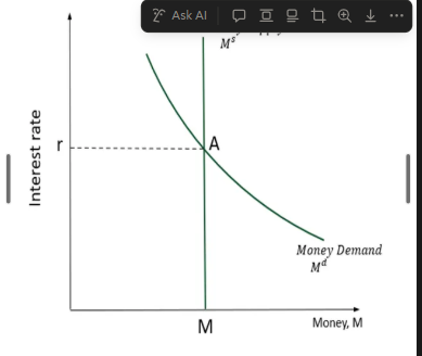
Determining the EQ IR: OMO:

• CB decides to supply an amount of money to public equal to M (currency*): Ms = M

• EQ in financial markets that requires Ms = Md = M (supply = demand)

• M = L (Y,r)

• Ms = fixed at some level

• Md = exogenous, determined by policy makers

• r = EQ IR

Commercial banks vs banks: 

Introducing Commercial Banks:

• CB chooses IR and then adjusted Money Supply to achieve target

• Banks: Financial intermediaries that have money in the form of deposits as liabilities

  • Keep some funds as reserves

  • Liabilities of CB = money it has issued (Central Bank Money) 

CB Assets	CB Liabilities	Bank Assets	Bank Liabilities
Bonds	Central Bank money	Reserves	Checkable deposits
	(includes reserves + currency)	Loans
		Bonds

Demand for Central Bank Money:

Demand for Central Bank Money:

Demand for deposits = Md = L (Y,r)

• Demand for CB Money = Demand for reserves by commercial banks (dependent on deposit demand)

H^d =𝜃𝑀^𝑑=𝜃𝐿(𝑌,𝑟)

• Demand for reserves = H^d

• 𝜃 = reserve ratio, the amount of reserve banks hold per £ of chequing deposit

Equalities for the demand of central bank money:

Equality: Hd = Md: demand for CB reserves by commercial banks is proportional to people’s money demand

Equality: Md depends on Y and IR </aside>

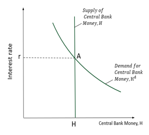
Determining IR: EQ in the market for Central Bank Money

r = fixed at some level, exogenous determination, EQ IR

• EQ IR is where Ms = Md

• Increase r decreases H (vice versa)

A = EQ 

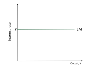
LM Model:

• LM in real terms: M / P = L (Y,r)

• CB chooses IR, so LM relation: r = ¯r </aside>

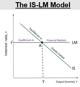
IS-LM model EQ and explanation:

• EQ in goods market implies increased IR reduces output (IS curve)

  • any point on the downward sloping IS curve = Goods market EQ

• EQ in financial markets = horizontal LM curve

  • any point on the horizontal LM curve = financial market EQ

• Both equilibria satisfied at point A

• Data suggests the model gives a sense of dynamic adjustment

• Observations are consistent with the implications of IS-LM model but does NOT prove that IS-lM is the right model

• Solid foundation for movement and activity in the SR

Q) Explain how an increase in government spending affects equilibrium output and interest rates in the IS–LM model. (4 marks)

• Identify policy:

  • Expansionary fiscal —> Increased G / Decreased T (vice versa)

• Effect on IS curve:

  • Expansionary —> IS curve shift right (vice versa)

• New Equilibrium:

  • Expansionary —> Increased output, decreased IR (vice versa)

• Reasoning:

  • Higher G / Lower T —> increased AD —> Increased Md = increased IR (movement along LM)

Q) Explain how an increase in the money supply affects equilibrium income and interest rates in the IS–LM model. (4 marks)

• Identify policy:

  • Expansionary monetary —> Increased Ms (vice versa)

• Effect on LM curve:

  • Expansionary —> LM curve shifts right/ down (vice versa)

• New Equilibrium:

  • Expansionary —> Decreased IR, Increased Output (vice versa)

    • (wants growth / expansion so cost of borrowing falls, output booms)

• Reasoning:

  • change in Ms impacts IR, influencing investment and AD

Q) Using the IS–LM model, explain how simultaneous expansionary fiscal and monetary policies affect equilibrium income and interest rates. (4 marks)

• Expansionary:

  • Fiscal: IS curve shifts right, increased Y, increased income ‘

  • Monetary: LM curve shifts right / down —> reduced IR, increased Y

• Combined effect:

  • Larger increase in Output, smaller change in IR depending on policy strength

Expansionary open market operation definition:

the central bank expands the supply of money by buying bonds and pays for it by creating money.

• Demand for bonds, Bond Price, Interest Rate ( Ms)

Contractionary open market operations: 

The central bank contracts the supply of money by selling bonds and removes from circulation the money it receives for the bonds.

• Demand for bonds, Bond Price, Reduces Interest Rate ( Ms)

IS-LM dynamics:

• Consumers are likely to take time to adjust consumption following a change in DY

• Firms are likely to take time to adjust:

  • investment spending following a change in sales

  • investment spending following a change in IR

  • production following a change in sales

The Empirical Effects of an Increase in the Federal Funds Rate:

• In the short run, a 1% increase in the federal funds rate —> decrease in output , increase in UN but has little effect on the price level.

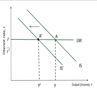
Covid-19 pandemic and the IS-LM Model impact: 

• Major policy-induced supply shocks

• Lockdown forced sectors (hotels, airlines etc.) to halt of slash supply

• Many firms had no choice other than to decrease / stop production, compared to other supply shocks like oil price rises where they could pass on costs

• Sharply lower output + Y + uncertainty —> impacted D in affected and non-affected (automobiles), sectors

  • shift left in IS curve and movement along LM, lower Y, constant r_

• Outcome: supply shock + sharp demand response

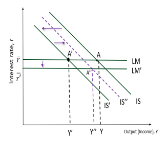
Covid-19 pandemic and the IS-LM Model response:

• Monetary-fiscal policy mix would have given Y”, but is absent so gives Y’

  • Could not increase output much but was necessary to save firms from bankruptcy / job losses

    • to limit effect of low-demand in non-affected sectors

• Fiscal response:

  • UK - furlough scheme, business grants, eat-out to help out

  • US, FRA, GER- subsidies, tax deferrals

• Monetary response:

  • IR were already very low, so CB took further measures

    • e.g. intervening in FM, providing funds to borrowers to increase lending

  • UK - Bank cut rate to 0.1%

Appendix - Bond prices and Interest rates formula

(Perpetual) bond price when market interest rate changes = Coupon Payment / r

£1000 face value, 10yr bond, 5% coupon rate, Annual coupon = £50

• If market interest rate stays at 5%: Price = 50/0.05 = £1000

• If market rate rises to 7%: 50/0.07 = £714.3

• If market rate falls to 3%: 50/.03 = £1666.7

Alternative EQ to Bond prices and IR with Required Yield:

Alternatively, market interest rate (Required yield) = Annual Coupon /Bond Price

Explain the Aggregate Demand Curve with P and Y as axis: 

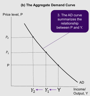
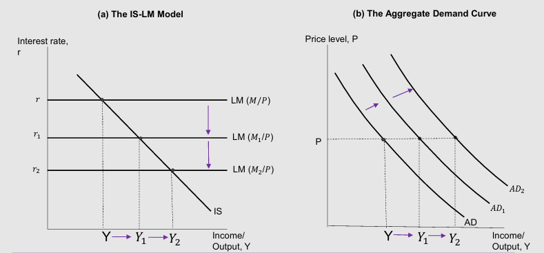
Monetary policy (IS-LM model) and AD curve:

• BoE can increase AD by adjusting r (vice versa)

• Decrease in r—> shift down in LM —> Higher M —> Increased I —> Increased Y at each value of P

• Increase in AD shifts out AD curve —> Increased Y at constant P

Aggregate Supply equation:

Y = Ȳ+ 𝛼(P - EP)

• Y = aggregate output

• Ȳ = natural rate of output

• 𝛼 = positive parameter

  • 𝛼 > 0; measures responsiveness of Y to unexpected changes in PL

• P = actual PL

• EP = expected PL

• Y and P are positively related so SRAS curve is upward sloping

Basis of Sticky-Price model with reasons for and assumptions: 

• Firms do not instantly adjust prices in response to demand changes

• Reasons for:

  • LT contracts between firms and customers

  • Menu costs

  • Firms wishing not to annoy customers with frequent price changes

• We ASSUME they set their own prices

To formalise the idea of sticky prices as the basis for upward sloping AS curve:

1. Consider pricing decisions of individual firms

2. Add together the decisions of many firms

Desired price level for an individual firm:

• Desire price for a flexible-price firm:

  p = P + a(Y - Ȳ)

• a > 0: firms raise prices when demand is high

Types of price firms:

• Flexible-price firms: set price using actual P and Y

• Sticky-price firms: set prices before knowing actual values

  p = EP + a(EY - EȲ)

• They expect output to be a its natural level

  • a (EY - EȲ) = 0 —> p = EP

Aggregate price level with sticky and non-sticky firms equation: 

• s = share of sticky-price firms

• (1-s) = flexible firms

P = EP + [(1-s)/s * a(Y - Ȳ]

• Higher EP —> Higher P (sticky firms set high prices early, flexible follows)

• Higher Y —> Higher P (flexible-price firms raise prices when demand is strong)

• Effect of output on prices is stronger when s is smaller

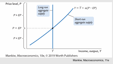
Deriving the AS curve:

• Y rises above natural Y when P > EP

• Sticky-price explanation for an upward-sloping SR AS curve.

• Solve for Y (SRAS Equation):

  Y = Ȳ + a(P - EP)

• Where:

  a = s / (1-s)a > 0

• P > EP —> Y > Ȳ

• P = EP —> Y = Ȳ

• P < EP —> Y < Ȳ

• derivations of Y from Ȳ are related to deviations of P from EP

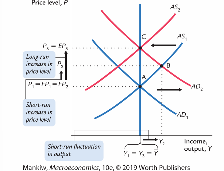
SRAS diagram:

• SRAS equation: Y =Ȳ+α (𝑷 −𝑬𝑷)

• SRAS curve: output is related to unexpected movements in P

• AD shifts out to AD2, SR fluctuation in output to Y2, new EQ of B, SR increase in P, AS1 constant

• AS1 shifts in to AS2, LR decrease in Y back to Y1, new EQ of C, LR increase in P, AD2 constant

• Policy makers aim to control INF and low UN, using F or M policy to expand AD —> along SRAS (lower UN, higher P)

  • evidenced by the Phillips Curve

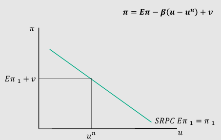
Phillips curve and what 𝝅 depends on: 

• Phillips Curve reflects the SRAs curve; as policy makers move economy along SRAS, INF and UN are inversely related and move

• 𝝅 depends on:

  • expected inflation: E𝝅

  • Cyclical UN: deviation (u) from natural rate (u^n)

  • supply shocks (v)

  𝝅 = E𝝅 - β (u - u^n) + v

• β > 0 is an exogenous constant measuring INF responsiveness to cyclical UN

Rational Expectations:

Rational Expectations: People base their expectations on all available information, including current and future policies

Adaptive Expectations and Inflation Inertia:

• Assumes people form their expectations of future inflation based on recently observed inflation

• E𝝅 = 𝝅-1

  Phillips Curve: 𝝅 = 𝝅-1 - β(u - u^n) + v

• Implies inflation inertia:

  • in the absence of supply shocks of Cyclical UN, inflation will continue indefinitely at its current rate

  • Past INF —> Current expectations —> Influences wages and prices

u^N (NAIRU): Nonaccelerating inflation rate of unemployment

• β = slope of Phillips curve

• SR curve depends on E𝝅

  • e.g. if it rises, SRPC shifts upwards, trade-off less favourable (higher 𝝅 for any UN level )

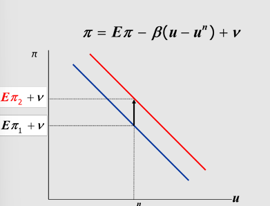
Phillips Curve inflation equation:

Phillips Curve: 𝝅 = 𝝅-1 - β(u - u^n) + v

Demand-pull inflation:

Demand-pull inflation

• Inflation resulting from demand shocks

• Positive shocks to AD: UN < u^n —> increases INF

• Negative shocks to AD: INF falls

Cost-push inflation: 

Cost-push inflation

• Inflation resulting from supply shocks

• Adverse supply shocks (v = +) —> increased production costs —> firms raises P —> Increased INF

• Favourable supply shocks decrease INF

Sacrifice ratio:

Sacrifice ratio

• To reduce INF, policymakers can contract AD → UN > u^n

Sacrifice ratio: measures the % of real GDP that must be forgone to reduce 𝝅 by 1%

• estimate = 5, for every 1% INF, 5% GDP must be sacrificed

• 4% decrease INF = 20% sacrifice of GDP

  • spread or rapid

  • cost of disinflation is lost GDP

Okun’s law: 1% increase in UN = 2% of lost output in real GDP

Why may the sacrifice ration be very small?

• Sacrifice ration may be very small due to rational expectations

  • People base their expectations on all available information, including current and future policies

• Gov announces desire to reduce 𝝅 from 6% to 2% ASAP

• Credible → E𝝅 will fall perhaps by 4% (as people expected 𝝅 to fall)

• 𝝅 can fall without an increase in u

Derive the AD schedule using the IS-LM model. Explicitly state any assumption(s) that must be made.

1. Derive the AD schedule using the IS-LM model. Explicitly state any assumption(s) that must be made.

• looking at real money balances

• Allowing price changes we can examine what happens to IS-LM model, price change shifts schedule and impacts income

• AD schedule captures relationship between price and income

• AD diagram + ISLM model

Explain the sticky price theory of aggregate supply. On what market imperfection does the theory rely?

2. Explain the sticky price theory of aggregate supply. On what market imperfection does the theory rely?

• explain the model of SRAS curve with equation 𝐘 = ̄ 𝒀+𝜶 (𝑷−𝑬𝑷)

  • attempts to explain why output might deviate from its natural level

    • occurs when P deviates from EP

• market imperfection is that prices do not adjust immediately to demand changes: explain

• Without full derivation: price-setting behaviour, implications- higher EP = higher P and higher Y = higher P, types of firms,

• Implications e.g. when P = EP, >EP, <EP

• SRAS diagram

3. Suppose the economy is initially at a long-run equilibrium. The Bank of England then reduces the base rate to increase the money supply. Assuming any changes in inflation to be unexpected, describe changes in GDP, unemployment and inflation that are caused by monetary expansion. Explain your conclusions using three diagrams: one for the IS-LM model, one for AD AS model and one for the Phillips curve.

3. Suppose the economy is initially at a long-run equilibrium. The Bank of England then reduces the base rate to increase the money supply. Assuming any changes in inflation to be unexpected, describe changes in GDP, unemployment and inflation that are caused by monetary expansion. Explain your conclusions using three diagrams: one for the IS-LM model, one for AD AS model and one for the Phillips curve

• LR EQ —> expansionary phase: ISLM model, LM shifts down, higher Ms, higher Y

  • LR impacts e.g. price rises, RMB original level, LM original position

• AD-AS model —> decrease r impacts

  • expansion raises E𝝅, SRAS shifts upward, economy Y natural level, higher P

• Phillips curve starts with u^n —> decrease IR increases Y above natural, u < u^n

  • movement along SRPC Hi INF low UN

  • Expansion raises E𝝅, SRPC curve upward —> higher 𝝅 and u^n

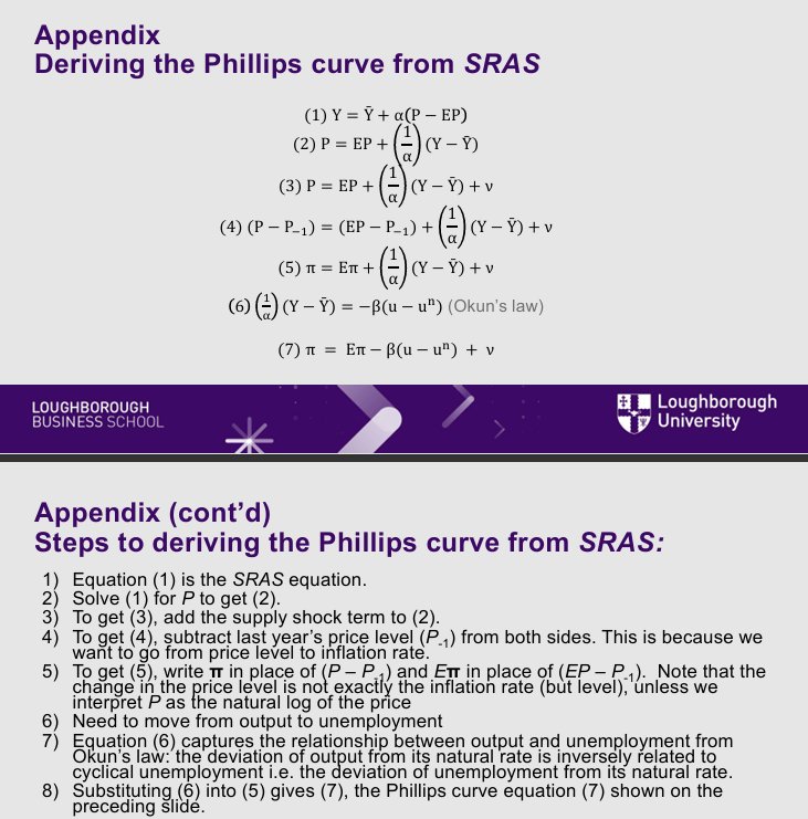
Deriving Phillips Curve from SRAS

1. Equation (1) is the SRAS equation.

2. Solve (1) for P to get (2).

3. To get (3), add the supply shock term to (2).

4. To get (4), subtract last year’s price level (P-1) from both sides. This is because we want to go from price level to inflation rate.

5. To get (5), write π in place of (P – P-1) and Eπ in place of (EP – P-1). Note that the change in the price level is not exactly the inflation rate (but level), unless we interpret P as the natural log of the price

6. Need to move from output to unemployment

7. Equation (6) captures the relationship between output and unemployment from Okun’s law: the deviation of output from its natural rate is inversely related to cyclical unemployment i.e. the deviation of unemployment from its natural rate.

8. Substituting (6) into (5) gives (7), the Phillips curve equation (7) shown on the preceding slide.

Mundell-Fleming model vs ISLM model:

Intro:

• Open economy extension affects both goods (IS) and money (LM) markets

• Assume fixed PL and show causes of SR changes in Aggregate Income (like ISLM)

• ISLM closed, key difference

Assumption of Mundell-Fleming Model:

• Small open economy with perfect capital mobility

r = r*

• r* = world interest rate (exogenously fixed)

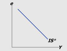
IS* Curve: Goods Market EQ equation and diagram: 

IS* Curve; GMEQ: Y = C(Y-T) + I (r*) + G + NX (e)

• e = nominal exchange rate = foreign currency per unit domestic currency

• IS* Curve is drawn for a given value of r*

• Slope intuition: decrease in e —> increase in NX —> increase in Y

• Lower ER (depreciation) —> domestic currency cheaper elative to foreign currency

• Increases NX —> exports (imports) relatively cheaper (more expensive)

• Increases demand for domestic output

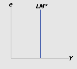
LM* Curve: Money Market Equilibrium equation and diagram: 

M / P = L (r* / Y)

• Real money balance = money demand

• L = liquidity reference

Md and Ms are independent of Exchange rate

• Vertical because only one value of Y will equilibrate the money market

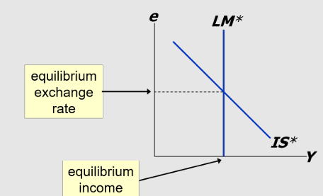
Equilibrium in the Mundell-Fleming model

Y = C(Y-T) + I (r*) + G + NX (e)

M / P = L (r* / Y)
Exogenous variables: G, T, P, r*

Endogenous variables: Y, e

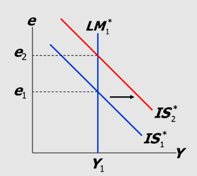
Fiscal policy under floating ER process (small open economy):

• M / P = L (r* / Y)

• Y = C(Y-T) + I (r*) + G + NX (e)

• At any given value of e, fiscal expansion increase Y, shifting IS* to the right

• Δe > 0, NX<0, ΔY = 0

• Increase G —> Increase Y —> IS1* shifts out to IS2* due to increase in demand for currency —> domestic investment is more attractive —> only temporary because more foreign demand for domestic currency —> fall in r* —> shifts to EQ at e2 level with Y constant

• Fiscal policy CANNOT affect real GDP

  • Crowding out: Small open economy: fiscal policy crowds out NX by causing exchange rate appreciation

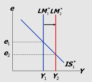
Monetary policy under floating ER diagram and impact(small open economy):

• Expansionary monetary policy shifts LM(right via impact on Ms) e1 shifts to e2, depreciation due to increase Ms as value of currency falls —> NX increase as exports are more attractive to foreign consumers due to cheaper prices —> Y must rise to restore equilibrium in the money market —> LM1 shifts out to LM2

• Δe < 0, NX>0**, ΔY** > 0

• Expansionary monetary policy does not raise world AD, it shifts demand from foreign to domestic products

  • increases in domestic income and employment are at the expense of losses abroad

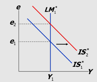
Trade policy under floating ER (small open economy):

• At any given value of e, tariffs or quotas reduce imports and increases exports —> increases NX and shifts IS* to the right

• domestic output increases —> Md increases —> upward pressure on domestic interest rates —→ e1 —> e2 appreciation

  • increased Q of loanable funds allows for a return from r —> r*

• Δe > 0, NX<0, ΔY = 0