Exam Key Explanations

Conditions for a Linear System

Linearity:

• 1. Amplitude scaling at input leads to amplitude scaling at output

• 2. Sum of two inputs gives sum of the two corresponding outputs

• 3. Zero input gives zero output

• 4. No new frequency components are generated

Conditions for a Time Invariant System

• No change in response due to a change in time of applying input

• If x(t) gives y(t) then x(t-t) gives y(t-t)

Relationship between time impulse and unit step

The impulse function δ(t) is the derivative of the unit step function u(t)

One direct and one indirect practical methods for determining the impulse response of a linear time invariant system.

Direct: apply a narrow pulse

Indirect: measure in the frequency domain and take the inverse transform

Causality

Causality means that the system response is zero if there is no input

That is the system is causal if h(t)= 0 for t < 0.

Stability

Stability means that if the input is bounded then the output is also bounded

That means that the integral (or the sum for discrete time systems) of the absolute value of the impulse response is finite

Four advantages of digital signal processing compared to analogue signal processing.

1. Signals and Systems are Stored in Digital Computers and Transmitted in Digital Form.

2. DSP is stable and reliable in Contrast to Analogue Components which drift with Temperature, Humidity, Time, Etc

3. DSP can be used to process a number of signals simultaneously (TDM)

4. Accuracy can be precisely controlled in contrast to analogue Systems where Component Tolerances and Inaccuracies Are Not Precisely Known.

5. More powerful DSP devices are becoming available at lower costs

6. When filters are implemented digitally they offer the following advantages:

(i) Practical and cheap filters for very low frequencies. Analogue filters require large components.

(ii) Frequency response can be made to approach the ideal more closely than analogue counterpart.

(iii) Adaptive filtering is readily achievable particularly with Microcomputers & Microprocessors

(iv) Filters with linear phase characteristics are possible.

Outline the necessary steps to implement the convolution of x(t) with y(t).

• Replace the independent variable with a dummy variable in both functions x(t) with y(t).

• Time reverse one of the two functions e.g. x(-t)

• Multiply the two functions x(-t).y(t)

• and find the area under the product. This gives the value of convolution at zero time shift

• Add a delay with the independent variable x(t-t)

• For each delay multiple the two functions x(t-t).y(t) and find the area under the product and this gives the value of convolution at t which is the original time variable.

• Repeat for all values of t until there are no common areas under the product.

• Convolution of two signals of duration T1 and T2 is equal to T1+T2

Give an example of a nonlinear system

A multiplier is a nonlinear system where the output has new frequencies. Similarly a squarer is a nonlinear system.

Four Applications of Spectrum analysis

1. Vibration analysis: Finding the resonances in a structure, string instruments, piano keys etc... such as in the L3 Vibrations course

2. Communications: Finding the spectrum of a signal forms the basis of communications theory. Without knowledge of the frequency range a signal occupies we cannot modulate it to transmit it in any form; that is no radio, no TV, no mobile phones, no internet, and no iPad…

3. Studying motor signals for example a drilling machine or a car engine does so many revolutions per second or per minute.

4. Studying human brain activity.

5. Music analysis.

6. Studying cyclic natural phenomena such as the diurnal cycle, the annual cycle, and the sun spot cycle which repeats every 11.4 years, and many more.

7. Finding the frequency response of mechanical and electronic systems such as the auditory system, filters used in limiting the frequency range of signals, mixers used to modulate signals to generate radio signals, engine response, gear box response, etc..

Symmetry Property of the DSS

An alternative to the SSS is the double sided spectrum DSS representing with positive and negative frequencies and complex coefficients which exhibit even symmetry in magnitude and odd symmetry in phase. This gives the double sided spectrum which for a real signal exhibits symmetry properties: even symmetry for the magnitude and odd symmetry for the phase.

What does a Type 0 system mean

Type 0, means no zero at the origin. Using final value theorem can find the steady state error of the system will not be zero

Steps for sketching root locus

• Decide system zero/poles and number of loci through number of zeros/poles;

• Mark zeros/poles;

• Where root locus starts from, and to where;

• Decide asymptotes and centroid using given equations from the formula sheet;

• Sketch the remaining parts.

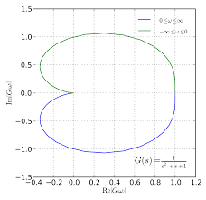
Nyquist Diagram

• Real Vs Imaginary Part as w varies

• Easy to know its absolute stability

• But difficult to choose key values of w

Nyquist Diagram: Real part vs Imag part as ω varies, easy to know its absolute stability; But difficult to choose key values of ω.

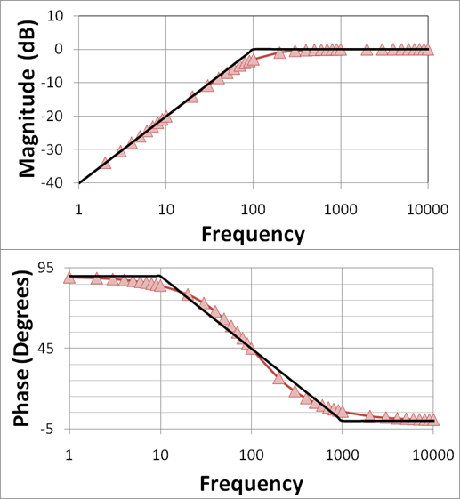
Bode Diagram

• Gain (dB) vs w and Phase (degree) vs w

• Large range of w

• Easily see the effects of controller design on PM and GM

• But two plots

Bode Diagram: Gain (dB) vs ω; Phase (degree) vs ω; Large range of ω; Easily see the effects of controller design on PM/GM. But two plots.

Compensation Design

Dynamic system itself may not directly satisfy required performance specifications. There often exist inherent trade-off among performance specifications. The purpose of compensation design is to meet more performance specifications, e.g., steady-state error, overshoot, and settling time.

Gain Compensator

Adding a gain compensator will not change original root locus, but can change stability, time response, and steady state error

Phase-lag compensator

Adding a phase-lag compensator will slightly change original root locus to the right of original root locus, making system tend to become unstable, but can reduce the steady-state error.

Phase-lead compensator

Adding a phase-lead compensator will change original root locus to the left of original root locus, making system become more stable, meeting more dynamic specifications.

State the difference between a practical phase-lead compensator and an ideal phase-lead compensator in terms of design procedure, implementation and their effects on system output.

• Implementation using different circuit such as RC, different method of choosing added zero location (ideal case by using angle criterion directly, and practical case by using own choice but instead choosing added pole by using angle criterion)

• Their time responses are also different in terms of overshoot and settling time etc.

• Ideal phase-lead compensator (also PD controller) is sensitive to step changes with input and sensitive to noise. Practical lead compensator can mitigate these effects.

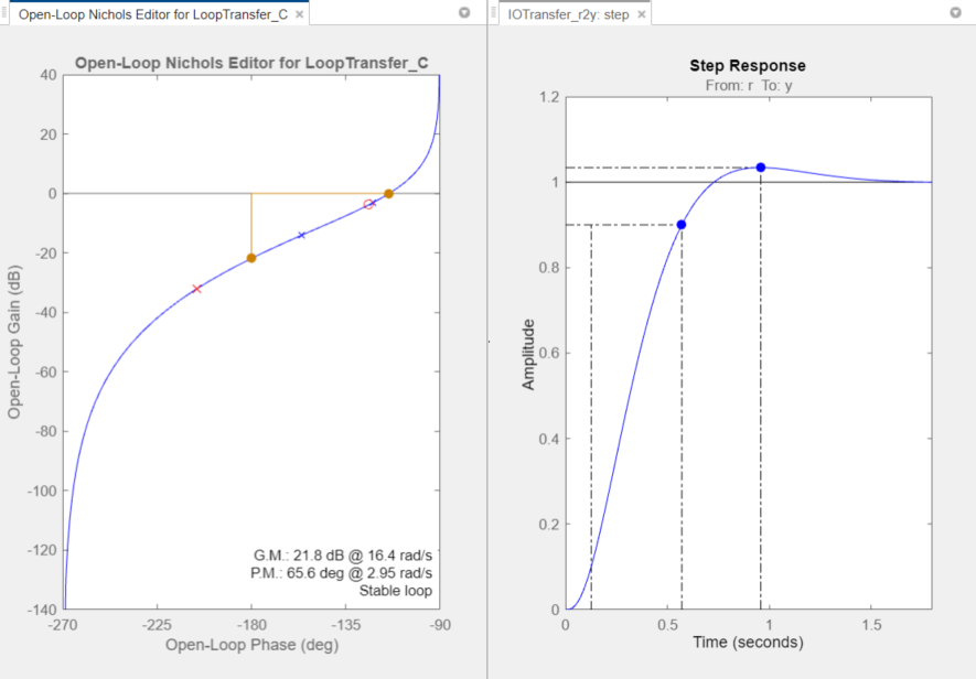
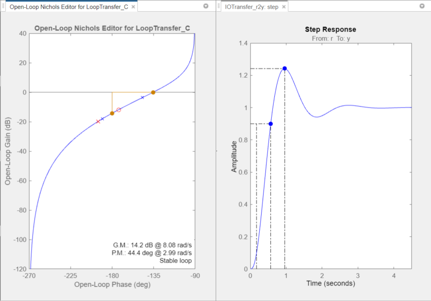
Gain margin

Gain margin is a factor by which the system gain can be increased before driving the system unstable.

Phase margin

Phase margin is the amount of additional phase lag that can be introduced into the system at the gain crossover frequency before making the system unstable.

State the meanings of gain margin and phase margin, and how you read them from Nyquist diagram and Bode diagram, respectively

• (i) Gain margin is a factor by which the system gain can be increased before driving the system unstable.

• (ii) Phase margin is the amount of additional phase lag that can be introduced into the system at the gain crossover frequency before making the system unstable.

• (iii) For finding gain margin, you need to find the phase cross-over frequency w_pi where the phase is -180 degree, the gain margin can be calculated by 1/|GH(i*w_pi)|.

• (iv) For finding phase margin, you need to find the gain cross-over frequency w_1, where the gain is unit. The phase margin is the difference between the phase of GH(i*w_1) and -180 degree.

Necessary steps of the root locus plotting.

• Decide system zero/pole and number of loci/lines, i.e., 3 lines

• Mark zeros/poles on s-plane, i.e., 0, -1,-0.25

• Show where root loci start from, and to where by arrows, i.e., starting from aforesaid poles, and going to infinity

• Decide asymptotes and centroids if there are lines going to infinity

• Sketch remaining parts using other rules.

Differences in closed-loop system vs open-loop system

Closed-loop system is robust to disturbance and change, more complicated with feedback loop and more expensive with extra components. Open-loop system is sensitive to disturbance and change, require recalibration but is cheap.

State the advantages of using the frequency domain approach over the time domain and s-plane approaches in the determination of system stability.

Problems with s-plane approach

• Root locus relies on the existence of OLTF, difficult to sketch for higher order system;

• Higher order systems ≈ second order, there exists an approximation error

Problems with time domain approach :

• Difficult to obtain or test;

• Computationally complex;

• Not easy to show the effects by graphical method

Advantages of frequency domain approaches :

• If TF known, FR can be directly known by s=jω;

• If TF unknown, FR can be obtained directly by experimental approaches;

• Easy to analyze effects of the system with sine signals (ready availability of various sine signal sources);

• Convenient to measure system sensitivity to noise and parameter variations (output frequency is the same as input frequency);

• Easy to measure relative stability by graphical method.

Nichols Chart

Nichols Chart: Gain (dB) vs phase as ω varies, Easy to read PM/GM; Similar but simpler plot than Bode diagram. But difficult to choose key values.

Difference Between Practical Phase-Lead and Phase-Lag Compensator

Feature	Phase-Lead Compensator	Phase-Lag Compensator
Objective	Improve transient response	Improve steady-state error
Design Principle	Add a zero closer to origin than a pole	Add a pole closer to origin than zero
Frequency Effect	Boosts gain at higher frequencies	Increases gain at lower frequencies
Effect on Phase Margin	Increases phase margin	Slightly decreases phase margin
Effect on Stability	Generally improves	May decrease if not designed carefully
Impact	Faster response, reduced overshoot	Better tracking, lower steady-state error

Forward vs Back Difference

Aspect	Forward Difference	Backward Difference
Substitution	s=z−1Ts = \frac{z - 1}{T}	s=1−z−1Ts = \frac{1 - z^{-1}}{T}
Stability	May map stable poles outside unit circle	Always maps left-half s-plane to inside unit circle
Accuracy	Less accurate for fast dynamics	More accurate and preferred for control

Advantages & Challenges of Digital Compensators

✅ Advantages:

• High design flexibility

• Easier to update or adapt (software updates)

• Noise immunity via sampling

• Lower implementation cost (no analogue hardware)

• Integration with microcontrollers / DSPs

⚠ Challenges:

• Sampling effects (aliasing, quantization)

• Requires fast ADCs/DACs

• Implementation of non-ideal delay

• Stability mapping between s and z domains

State the meanings of gain margin and phase margin. Explain how you read them from a Nichols Chart.

• Gain margin: How much gain can increase before instability → measured at phase = -180°

• Phase margin: Additional phase lag required to reach -180° → measured at gain = 0 dB

• On Nichols chart:

  • Find point where magnitude = 0 dB → read phase margin

  • Find point where phase = -180° → read gain margin

Give four applications of spectrum analysis

• Wireless communication

• Audio processing

• Vibration analysis

• Radar and Sonar Signal Processing

Symmetry property of the double sided spectrum

For real valued signals

• Magnitude spectrum is even symmetric: |X(-w)|=|X(w)|

• Phase spectrum is odd symmetric < X(-w)

Difference between a continuous and a discrete time signal

• Continuous defined for all t E R (analogue)

• Discrete defined only at n E Z (sampled)

• Continuous use integrals, discrete uses sums

• Different mathematical tools (FT vs DTFT/DFT)

Analysis and synthesis of signals and systems

Analysis: Decomposing signals/systems into fundamental components

Synthesis: Reconstructing signals/systems from components

Fourier analysis (Decomposition)

Fourier Synthesis (Reconstruction)

System analysis examines properties

Synthesis designs systems

P controller

P Controller (Proportional Controller)

The proportional (P) controller applies a control signal directly proportional to the error signal. Mathematically, the controller output is expressed as: u(t) = Kpe(t) where Kp is the proportional gain, and e(t) is the error signal.

Characteristics:

• Equivalent to a gain compensator.

• Improves the response speed.

• Reduce but does not eliminate steady-state error.

• Excessive Kp can lead to oscillations or instability.

Applications: Used in systems where steady-state error is acceptable but fast response is desired, such as pressure and temperature control

PI Controller

PI Controller (Proportional-Integral Controller)

The PI controller introduces an integral term to eliminate the steady-state error: u(t) = Kpe(t) +Ki e(t)dt where Ki is the integral gain.

Characteristics:

• Equivalent to a phase-lag compensator.

• Eliminates steady-state error by accumulating past errors.

• Can destabilize the system with a higher overshoot.

Applications: Commonly used in industrial control systems such as motor speed control and robotic manipulators, where steady-state error must be eliminated.

PD Controller

PD Controller (Proportional-Derivative Controller)

The PD controller adds a derivative term to predict future system behavior and enhance stability: u(t) = Kpe(t) +Kd d dt e(t) where Kd is the derivative gain.

Characteristics:

• Equivalent to a phase-lead compensator.

• Reduces overshoot and improves stability.

• Sensitive to noise due to derivative action.

Less effective for systems with significant disturbances or measurement noise because these will be amplified by this controller.

Applications: Used in motion control systems, such as robotic arms, where fast response with minimal overshoot is required.

PID Controller

PID Controller (Proportional-Integral-Derivative Controller)

The PID controller combines the benefits of P, I, and D terms to achieve a balanced performance: u(t) = Kpe(t) +Ki e(t)dt+Kd d dt e(t)

Characteristics:

• Equivalent to a lead-lag compensator.

• Removes steady-state error while improving stability and transient response.

• Requires tuning of three parameters: Kp, Ki, and Kd.

• Can be implemented in both analog and digital systems.

Applications: Widely used in industrial automation, process control, and aerospace systems where precise and stable control is essential.