Stats Year 1

Hypothesis testing

The use of statistical techniques to test a particular claim (the hypothesis). A sample from the population is used to see if the result from the sample is consistent with the claim.

Process of a hypothesis test - Set up/ state the hypotheses

the null hypothesis (H₀) - where p takes a particular value/ the value you would expect

alternative hypothesis (H₁) - the probability you’re testing (one-tailed or two-tailed?)

Process of a hypothesis test - Setting the significance level

This is the probability of rejecting the null hypothesis if in fact it is true

Process of a hypothesis test - Carrying out the test (P-values)

Use a sample to obtain a test statistic (the value of X in X ∼ B(n,p))

probability of obtaining a value at least as extreme as the test statistic, if the null hypothesis is true
For X has a value, use X ∼ B(n,p) to calculate…

• P(X > x) if H₁: p > x

• P(X < x) if H₁: p < x

• 2 x P(X > x) if H₁: p ≠ x

Whether the value of X given is in the critical region will determine whether to reject the null hypothesis.

Process of a hypothesis test - Carrying out the test (Critical regions)

Use a sample to obtain a test statistic (the value of X in X ∼ B(n,p))

set of values for the test statistic X for which you would reject the null hypothesis. The critical value is the value for X for which you change from not rejecting the null hypothesis to rejecting it.

• For H₁: p > x, use X ∼ B(n,p) to find the lowest value for r for which P(X > r) is less than the significance level.

• For H₁: p < x, use X ∼ B(n,p) to find the highest value for r for which P(X < r) is less than the significance level.

• For H₁: p ≠ x, the critical region has 2 parts to it, Split the significance level into 2, one for the lower tail and one for the upper tail. Then use X ∼ B(n,p) to find the lowest value for r for which P(X > r) is less than half the significance level and to find the highest value for r for which P(X < r) is less than half the significance level.

Whether the value of X given is in the critical region will determine whether to reject the null hypothesis.

Process of a hypothesis test - The conclusion

Reject H₀ - if p-value is less than sig level/ test statistic lies in critical region → there is sufficient evidence to suggest that H₁ is true

Not reject H₀ - if p-value is more than sig level/ test statistic doesn’t lie in critical region → there is not sufficient evidence to suggest that H₁ is true

Process of a hypothesis test order - 1

Set up/ state the hypotheses

Process of a hypothesis test order - 2

Setting the significance level

Process of a hypothesis test order - 3

Carrying out the test

Process of a hypothesis test order - 4

The conclusion

One-tailed test

When you think a result is more likely H₁: p > x

When you think a result is less likely H₁: p < x

Two-tailed test

When you think there’s a bias in general H₁: p ≠ x

Uses of binomial distribution

to model situations in which: you are carrying out trials on random samples of size n; there are 2 possible outcomes, success (where probability p is fixed) and failure; trails are independent of each other

Binomial distribution notation

X ~ B(n,p) where X is the number of successes, n is number of trials, p is probability

P(X = r) = ⁿC_r p^r (1-p)^n-r

Cumulative binomial probability

the probability of a range of results, written as P(X < 5)

Mean or expectation of a binomial distribution calculation

np

Experiment/ trial

Any situation involving uncertrainty

Outcome

the result of a trial or experiment

Sample space

The set of all possible outcomes of a trial or experiment

event

can be used to describe one or more possible outcomes from a trial or experiment

Mutually exclusive events

2 events that can never occur together. This means P(A U B) P(A) + P(B)

Independents events

When the occurrences of on of 2 events has no effect on the other occurring. This means P(A U B) P(A) x P(B)

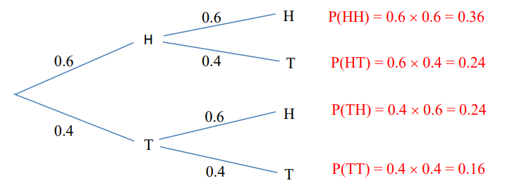
Tree diagram

Shows the outcomes of events and the probability of the outcome happening. Useful when dealing with events that have just 2 or 3 possible outcomes.

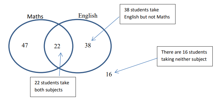
Venn diagram

Shows the outcomes of events and the probability of the outcome happening in combination with other events. Useful when dealing with events that are not mutually exclusive.

Simple random sampling

The items in the sample are chosen by a random process such as drawing from a box. Every member of the population has an equal chance of being selected

Opportunity sampling

Choosing individuals for a sample as opportunity arises, such as interviewing passers-by

Systematic sampling

Involves selecting individuals from a population by a systematic method, such as selecting every 10th individual on a list of the population

Stratified sampling

Used when the population can be divided into subgroups (strata) using criteria such as age or gender, and ensures that all strata are represented in the sample. Sometimes there is a requirement that the numbers sampled from each stratum is proportional to the sizes of the strata (this is called proportional stratified sampling). Otherwise, weighting is used

Quota sampling

Used when the population can be divided into strata. A certain number of items from each stratum are required

Cluster sampling

Used when the population consists of subgroups which are each reasonably representative of the population (e.g. year 6 classes in several schools). A sample is taken from just a few of these subgroups

Self-selected sampling

Used when individuals choose to be part of a sample, e.g. a survey posted on the internet

Mean x̄

A measure of central tendency found by adding up the data items and dividing by the number of data items

Median

A measure of central tendency that is the midpoint of the data when they are placed in numerical order

Mode

A measure of central tendency that is the most frequently occurring data value

Range

A measure of variation that is the difference between the highest and lowest values from the data

Interquartile range

A measure of variation that is the difference between the upper quartile (3/4 of data) and lower quartile (1/4 of data).

Variance

A measure of variation which is the measure of the spread of the sample

Variance equation

= (Σx_i² - nx̄²) / (n-1)

Standard deviation

A measure of variation is the square root of the variance

Bivariate data

Data which involves 2 variable e.g. height and weight

Positive correlation

Positive gradient of the line best of fit of bivariate data

Negative correlation

Negative gradient of the line best of fit of bivariate data

Outliers

An unusually high or low value in a data set. They are either any data value which is more than 2 standard deviations away from the mean or any data value which is more 1.5 times the interquartile range above the upper quartile or below the lower quartile.

Cleaning data

dealing with missing data, errors and outliers. How you deal with these issues depends on the situation and what you are using the data for