3. Finite Volume Methods

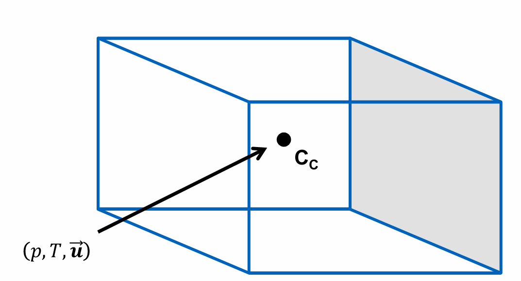
Describe how Finite-Volume Method is used to discretise a generic 3D polyhedral cell

• flow variables (p, T, u) vary linearly across the cell

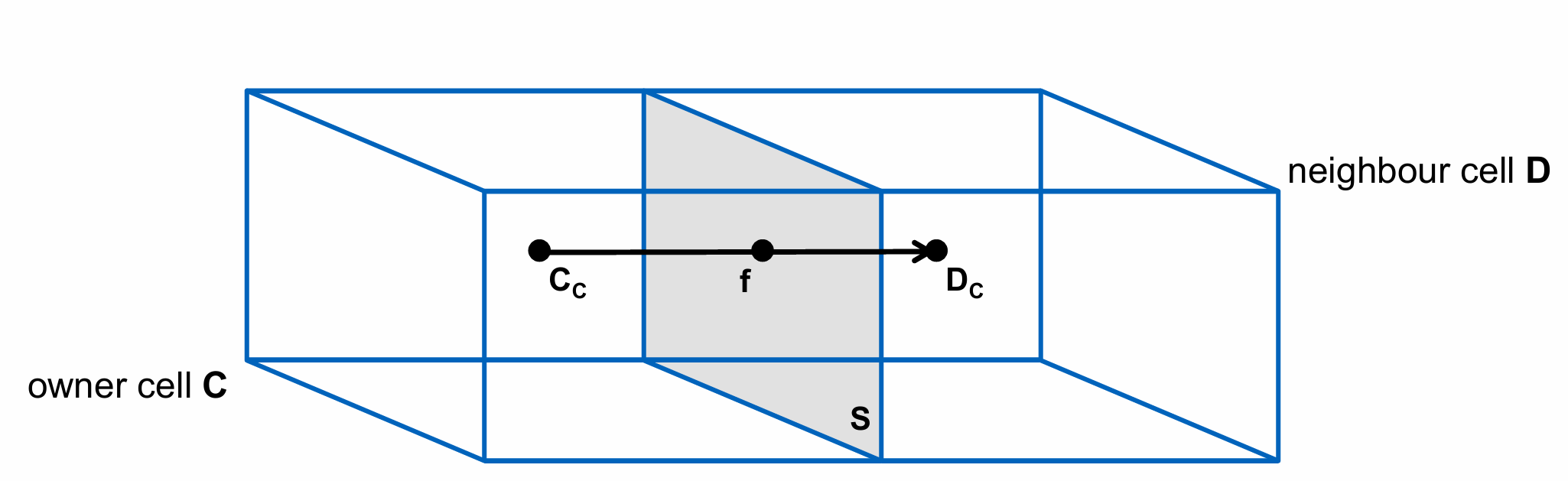
• flow variables are calculated at the cell centroid C_c, C_d

• cell has a volume V_c

• The location where the vector \overline{C_{C}D_{C}} intersects face S is the face center 𝑓.

\int_{V}\left\lbrack\nabla\cdot\left(u\cdot u\right)+\frac{1}{\rho}\nabla p-\nabla\cdot\left(v\cdot\nabla u\right)-g\right\rbrack dV=0

\int_{V}\left\lbrack\nabla\cdot\left(u\cdot u\right)\right\rbrack dV=\int_{V}\left\lbrack-\frac{1}{\rho}\nabla p\right\rbrack dV+\int_{V}\left\lbrack\nabla\cdot\left(v\nabla u\right)\right\rbrack dV+\int_{V}\left\lbrack g\right\rbrack dV

→ We need them in the following matrix form for the SIMPLE algorithm:

\overline{M}u=b

where

\overline{M} is a matrix of coefficients

What is a typical constant source term ?

→ gravity

\int_{V}\left\lbrack g\right\rbrack dV=gV_{c}

Considering the matrix form, we append the gravity force to the right-hand side (b vector)

\overline{M}u=b

How is a linear source expressed in the Navier-Stokes Equations?

\int_{V}\left\lbrack Su\right\rbrack dV=S_{C}u_{C}V_{C}

2 options:

1) We add -S_{C}V_{C} to the \overline{M} matric (implicit treatment)

2) We add S_{C}u_{C}V_{C} to the b vector (explicit treatment)

\overline{M}u=b

How do we solve the Convection Term of the Navier Stokes Equation across the cell (C)

• We use the divergence theorem to convert the volume integrals to surface integrals

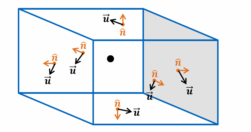
• The dot product of the velocity, the unit normal vector and the surface element results in the volume flow rate out of the surface

• The other velocity outside the bracket u is the unknown we are solving for

• The velocity is transported by the volume flux

• We can approximate the value at the face centre (f)

\sum_{f=1}^{_{}N}\int_{S}u\left(u\cdot n\right)dS_{f}=\sum_{f=1}^{_{N}}u_{f}\left(u_{f}\cdot n_{f}\right)S_{f}

How do we solve the Diffusion Term of the Navier Stokes Equation across the cell (C)

\int_{V}\left\lbrack\nabla\cdot\left(v\cdot\nabla u\right)\right\rbrack dV=\int_{S}\left\lbrack v\left(\nabla u\right)\cdot n\right\rbrack dS=\sum_{f=1}^{N}v_{f}\left(\nabla u\right)_{f}\cdot n_{f}\cdot S_{f}

• velocity gradient \left(\nabla u\right)_{f}

• kinematic viscosity v_{f}

What is face non-orthogonality

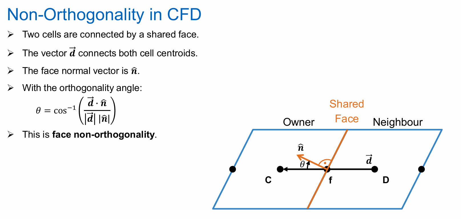
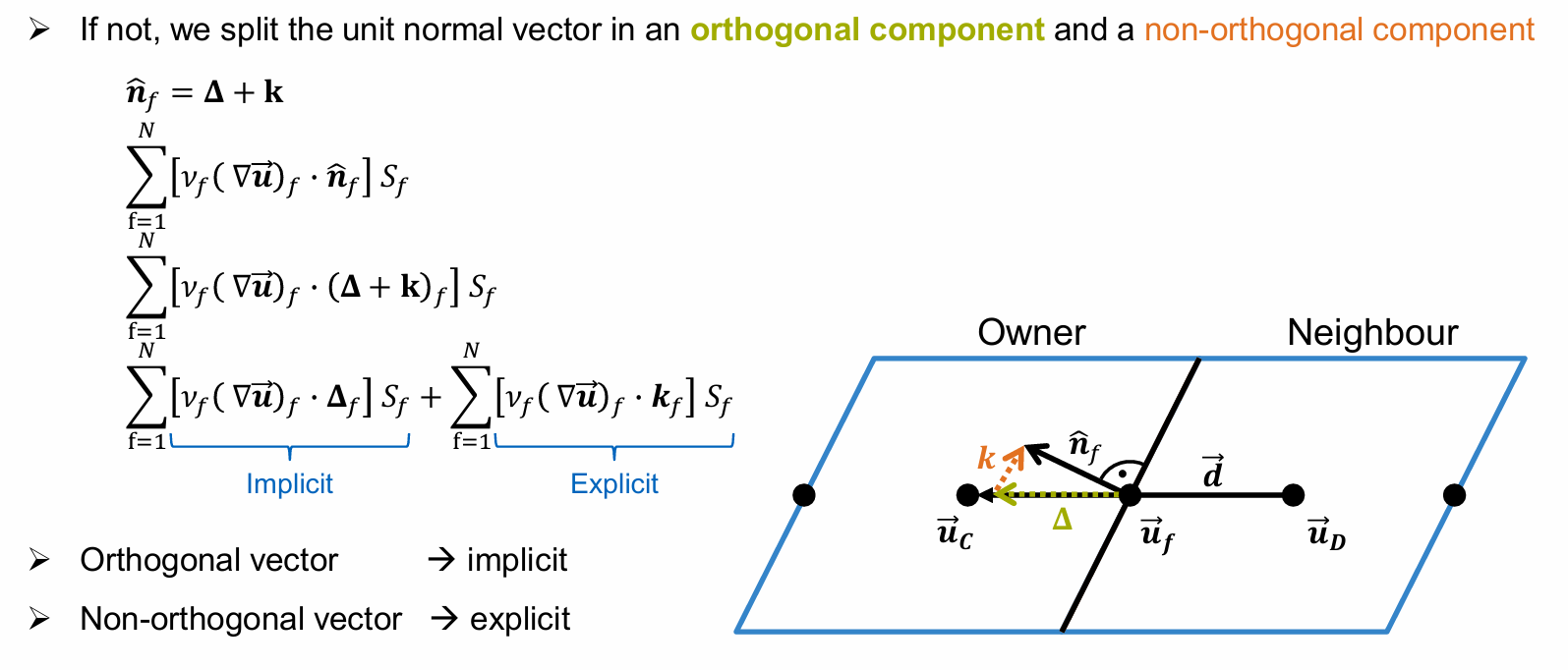
What do the orthogonal & non-orthogonal components of unit normal vector ?

Orthogonal Component → implicit → Term increases stability

Non-orthogonal components → explicit → Term decreases stability

The higher the non-orthogonality of the mesh:

• The larger the explicit term

• The smaller the implicit term

How do we solve the Navier-Stokes Equations numerically?

→ SIMPLE algorithm

\overline{M}u=b

Steps:

1. Solve the momentum equation for the velocity field. This velocity field does not satisfy the continuity equation

\overline{𝑀}𝒖=-𝛻p , Separate M into diagonal 𝑨 and off-diagonal 𝑯 components: 𝑀 𝒖 = 𝑨 𝒖− H

2. Solve the Poisson equation for the pressure field

𝛻\cdot\left(\overline{A}^{-1}𝛻p\right)=𝛻\cdot\left(\overline{A}\overline{^{-1}H}\right)

3. Use the pressure field to correct the velocity field so that it satisfies the continuity equation

u=\overline{A}\overline{^{-1}H}-\overline{A}^{-1}𝛻p

4. The velocity field now does not satisfy the momentum equations. Then repeat the cycle