Point Operators

Definition of point operator

an operator where pixel output values depend on the input value of that pixel and, optionally, global statistics

The point operator is a function (operator) of the following form:

g(x) = h(f(x))

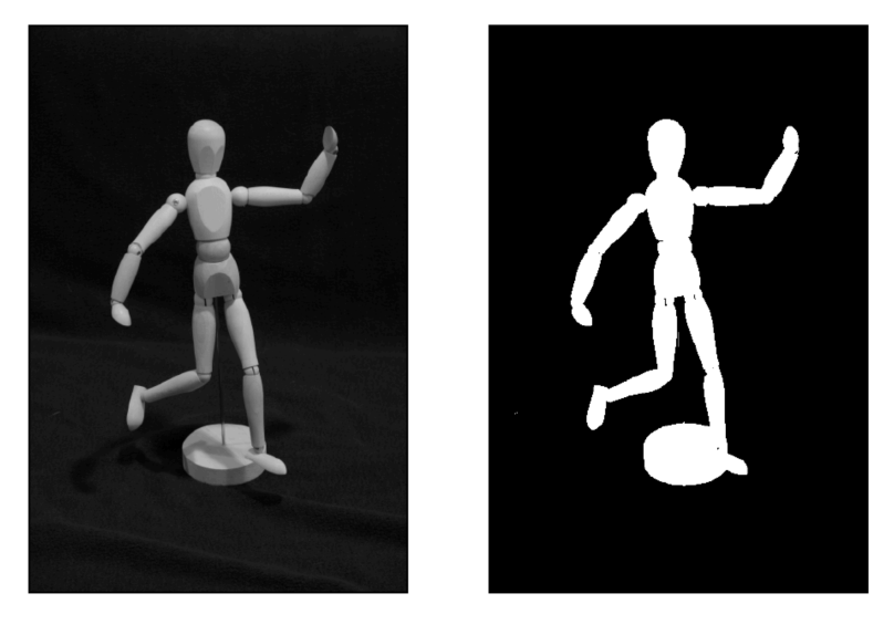
inversion

Consider pixel of grey-scale image with intensity w ∈ [0,1]

For inversion the point operator is h : w ↦ 1 − w

(“↦” is the “maps-to” symbol)

Simpler notation: h(w) = 1 − w

thresholding

Consider pixel of grey-scale image with intensity w ∈ [0,1]

An example thresholding operator:

w ↦ { a, for w ≤ 0.5

1, for w > 0.5

Computing contrast

Michelson: CM ( I ) = max ( I ) − min ( I ) / max ( I ) + min ( I )

RMS: CRMS = CRMS=1/MN SQRT(​u=0∑N−1​v=0∑M−1​(Iuv​−Iˉ)^2)

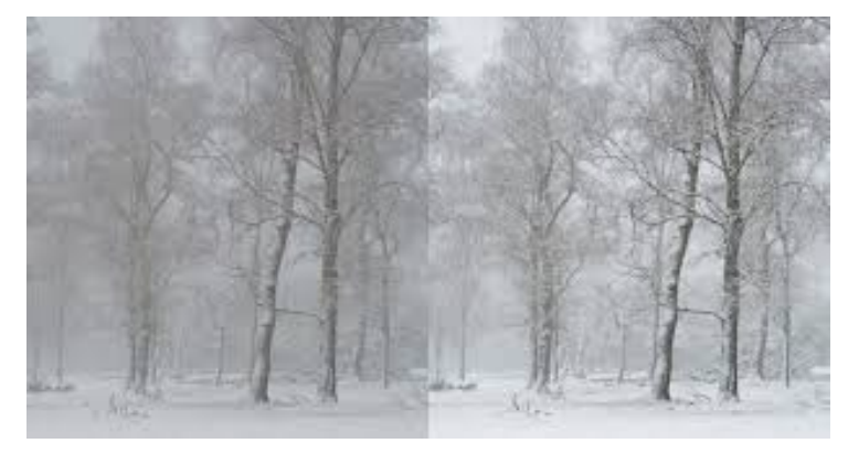
Adjusting contrast

Power law:

w′ = w^γ

Logarithmic transform:

w′ = log w

histograms

Many point operators are based on histograms

Simple for discrete-valued pixel values, e.g. w ∈ {0,⋯,255}

w ∈ {0,⋯,255}: h(i) = card{x | f(x) = i}, where x = [u, v]

In words: count the number of times a value occurs in the image

probability

Probability mass function (pmf): for discrete variable, e.g., x ∈ {0,1,⋯,255}

1. Probability mass function of (discrete) pixel intensity

Probability density function (pdf): probability x ∈ [a, a + ϵ]

1. For continuous variables

2. Because values have zero probability

3. ϵ very small

4. Probability density of wind speed

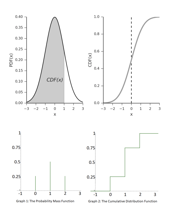
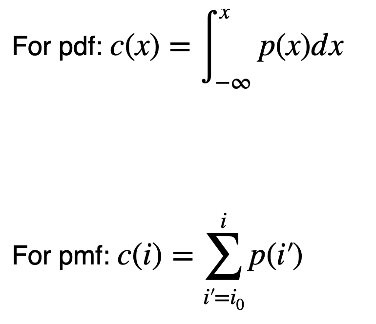
cumulative distribution function

Inverse cumulative distribution functions

Consider discrete valued case with pmf p(j) and j>=0

The cumulative distribution function (cdf) is:

c(i) = j=i ∑ j=0 p(j)

As the probabilities are nonnegative must be monotonically increasing.

As the cdf is monotonic, we can define its inverse c^-1

Inverse is unique if c is strictly monotonic. In any case we can define one if it is monotonic. For simplicity we will assume it is unique.

Let C be the probability that j ≤ C, then j = c^−1 (C)

Image histograms and the image pmf

An image histogram function h is an unnormalised empirical pmf

The values of h sum to the total number of pixels N

So p(i) = h(i)/N, where N is the number of pixels

As a vertical scale of the cdf we can use the pixel count instead of the empirical probability

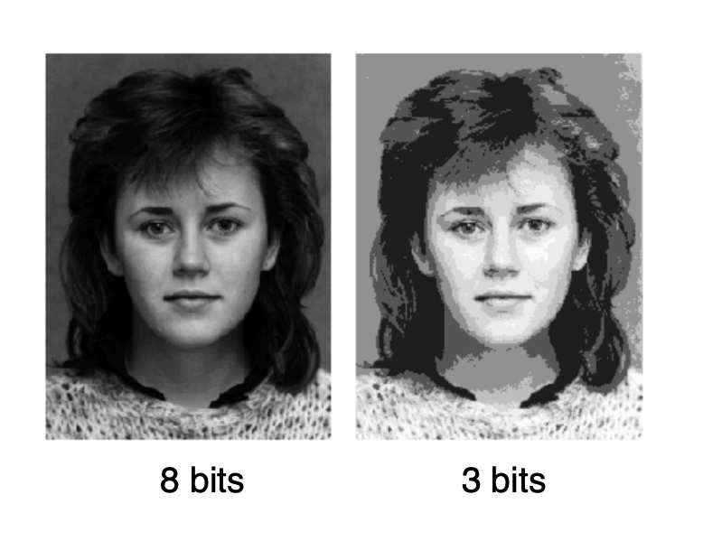
Quantisation

Pixel-wise quantisation is a simple (cheap) form of lossy compression

Poor compression efficiency

Uniform quantisation: j′ = α round( x / α ) α = quantisation step size (e.g. how far apart the quantised levels are)

Codebook based: q(m), m ∈ {0,⋯, M} j′ = q(m), m = arg min m (j − q(m))^2

Finds nearest codebook entry

Store index for each codebook entry

Exploit perception

We are more sensitive to luminance: natural to separate luminance and chrominance (e.g., YCbCr) and provide different scalar bit allocations

Exploit vector quantisation

Example of two-colour flower and VQ.

VQ more efficient than scalar quantisation.

Scalar quantisation particularly inefficient for example.

(Still a point operator.)