week 5: within measures ANOVAS

Repeated measures design

There are many situations in which we might want to study the same individual under several different conditions.​ Experimental design of this kind are called Repeated Measures Design (or related design or within-participants design).​

within measures ANOVA

or related, and not independent groups​

also referred to as a within-subjects ANOVA​

​

advantages of within measures design

it increases statistical power-the design removes the effects of individual differences

fewer participants are needed for most experiments-a big advantage if data is difficult to obtain because we cannot find the participants for our experiment

disadvantages of within measures design

the independent variable may be confounded with order of testing or carry over effects:

1. Practice Effects ​

subjects get better at the task over time because of practice, so that they perform best in the later conditions​

2. Fatigue Effects ​

subjects get worse at a task over time because of fatigue, so they perform worse in the later conditions​

3. Contrast Effects ​

a noisy condition experienced after a quiet condition might be perceived as even noisier than it normally would be. ​

4. Demand Characteristics​

being in more than one condition makes it clear to subjects what the independent variable is. They may behave how they think you want them to in later conditions

missing data

solutions to order effects

Randomising the order of testing

Counterbalancing order of testing

F calculation

between-groups variance (with indiv. diffs. removed)/within groups variance (with indiv.. diffs. removed)

ANOVA assumptions

• The Dependent Variable (DV) comprises data measured at interval/ratio level. ​

• Use Kolmogorov-Smirnov or Shapiro-Wilk tests to confirm normal distribution.​

• At least three (or more) measurements from the different conditions/treatment isrequired.​

• All participants the provide score for all the conditions/treatments.​

• Homogeneity of Variance- Use Mauchly’s Test of Sphericity (within measures design).​

sphericity

Sphericity means that the variances of the differences between all combinations of related groups (levels) are equal/same. ​

Violation of sphericity is when the variances of the differences between all combinations of related groups are not equal/same. ​

Sphericity replaces the homogeneity of variance assumption in independent measures ANOVA

if the assumption of sphericity is not met, All is not lost. SPSS gives us some other decisions….. We have estimate of sphericity. ​

• Greenhouse-Geisser – conservative (if epsilon is < 0.75). ​

• Huynh-Feldt – least conservative (if epsilon is > 0.75).​

• Lower-bound – most conservative (least reported).

most commonly use greenhouse-geisser

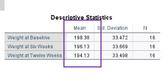
descriptives

A quick glance at the Descriptives Statistics shows us that there is a linear trend in weight loss over the twelve-week period. ​

The mean weight decreases from 198.38(Weight at Baseline) to 196.13 (Weight at Six Weeks) to 194.13 (Weight at the end of period).

degrees of freedom

weight df=no. of conditions-1

error (weight) df=(no. of observations-1)-(no. of participants-1)-(no. of conditions -1)

mean square

mean square=sum of squares/degrees of freedom

error mean square=error sum of squares/error df

F ratio

mean square/error mean square

evalaute null hypothesis

e.g. =35, the observed variance is 35 times which is a substantial difference

effect size

eta squared

planned comparisons

• we have hypothesised in advanced which meanswill differ from one another before we start the experiment.​

• In this example, we hypothesised that there will be a difference in the body weight over the 12-week period. ​

• Furthermore, we predicted that there would be a difference between ​

(a) Baseline and Mid-Point (six weeks) and ​

(b) Mid-Point (six weeks) and End Period (twelve weeks).

Planned contrasts showed that there was a significant difference between the mean weight at Baseline whencompared to mid-point (6 Weeks), F(1, 15) = 13.65, p=0.002, partial ŋ2 = 0.48 indicating a difference of 48% in theweight loss between the Baseline and six weeks. This is large effect size.​​

unplanned (post-hoc) comparisons

If this was a speculative study and it was not possible to predefine your hypothesis, you could conduct a post-hoc comparison of all the mean differences in SPSS.​

Remember that unplanned tests are less scientifically rigorous.​

Give the means, SDs and significance levels for mean comparisons​

Unplanned contrasts with Bonferroni adjustment identified that mean weight was significantly lowerat Week Six (M= 196.13, SD = 33.67) than at Baseline (M=198.38, SD=33.47, p=0.006) and Week 12(M=194.13, SD = 33.50) than at Baseline (M=198.38, SD=33.47, p<0.001) and Week 12 (M=194.13,SD=33.50) than Week Six (M=196.13, SD=33.67, p=0.001)

also report effect sizes (cohen’s d)