Econ 102 - CHAPTER 11: The Labor Market

Labor Market

Supply

Workers (sell labor)

As wages ↑ → more hours worked

Upward-sloping

Demand

Businesses (buy labor)

As wages ↓ → more workers hired

Downward-sloping

Wage = price of labor; hours = quantity.

Marginal principle

Break a “how many” question into a “one more” question

Ex:

Should I hire one more worker

Cost-benefit principle

Does the marginal benefit exceed the marginal cost? If yes, then do it!

 Marginal cost of one more worker
the additional wage you now must pay this worker.

 Marginal benefit
he extra revenue you get from the extra stuff they produced for you.

Marginal Product of Labor (MPL)

Extra output from hiring one more worker

Marginal Revenue Product (MRPL)

Extra revenue from hiring one more worker

Rational Rule (Employers)

Hire until wage = MRPL (Marginal Revenue Product of Labor)

Rational Rule (Workers)

Work until wage = MB (Marginal benefit) of leisure.

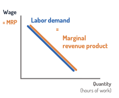
Labor Demand Curve

• Downward sloping: higher wages → fewer workers hired.

• Same as MRPL curve (extra revenue per worker).

Labor Demand Shifters

1. Change In demand for product ↑ → labor demand ↑ (derived demand).

2. Changes in price of capital (machines):

   • ↓ Price of capital →

     • Scale effect: expand output → hire more workers.

     • Substitution effect: replace workers with machines.

     • Outcome depends on which effect dominates.

     • If scale > substitution → complements (↑ demand).

     • If substitution > scale → substitutes (↓ demand).

3. Productivity/Technology improvements: workers become more valuable → ↑ demand.

4. Non-Wage costs (benefits/taxes): ↑ costs → ↓ demand; ↓ costs → ↑ demand.

Scale effect (Demand Curve)

When the price of capital
declines (or any input gets cheaper), you
can now produce at a lower cost. This
encourages you to produce at a larger
scale, which may require more workers.

More machinery and workers

• Labor demand increases (Shift right)

Substitution effect (Demand Curve)

Many tasks can be
done by either workers
or machines.
When the price of machines falls, the
company will replace workers with the
cheaper machinery.

Greater use of machinery, replace workers

• Labor demand decreases (shift left)

Labor Supply Curve

Upward sloping

1. High wages attract new workers.

2. Current workers work more hours.

3. People switch occupations for better pay.

Labor-Leisure Trade-Off

• Opportunity cost principle: every hour of work = one less hour of leisure.

• Decide how to allocate 24 hours to maximize happiness.

When the wage rises, there are two different effects

The Substituion or Income effect

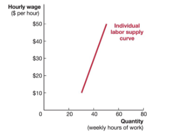
Substitution Effect (Supply)

When your wage goes up, the opportunity cost of an hour of leisure goes up.

• You now forfeit more money when you
  take an hour of leisure.

• Higher wages are an incentive to substitute toward work and away from leisure

If the substitution effect dominates, then the high
wage has provided a stronger incentive for you to work.
 As wage rises, you work more hours.
 Labor supply curve slopes upward

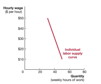
Income effect:

A higher wage increases
your income, leading you to choose more
leisure and hence less work.

• Leisure is a normal good, and people
  consume more normal goods when
  their income increases.

• Thus, under the income effect, a higher
  wage leads you to work fewer hours

If the income effect dominates, then a high wage raises
your income and you “spend” this extra income buying
more leisure
 As wage rises, you work fewer hours.
 Labor supply curve slopes downward.

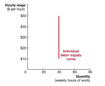
If the income and substitution effects offset

then your incentive to work more hours is perfectly counter balanced
by your incentive to work fewer hours.
 As wage rises, you do not change your hours worked.
 Labor supply curve is perfectly vertical

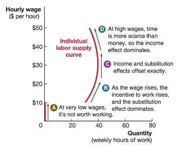
If the dominant effect changes as wage changes, then the labor supply curve takes a

backward-bending shape.

 At lower wages, the substitution effect dominates, resulting in an upward slope.
 At mid-range wages, the two effects offset, resulting in a vertical slope.
 At higher wages, the income effect dominates,
resulting in a downward slope

Labor Supply Shifters

• Wages in other occupations: higher elsewhere → ↓ supply here.

• Number of potential workers: ↑ population → ↑ supply.

• Benefits of not working: higher benefits (college aid, unemployment) → ↓ supply.

• Nonwage benefits/taxes:

  • ↑ benefits or ↓ taxes → ↑ supply.

  • ↓ benefits or ↑ taxes → ↓ supply.

Three-step recipe for analyzing the labor market

Determine which curve is shifting:

1. labor supply, labor demand, or both

2. Determine if the shift is an increase or a decrease.

3. Determine how wages and number of jobs will change in the new
   equilibrium