4A9 molecular thermo

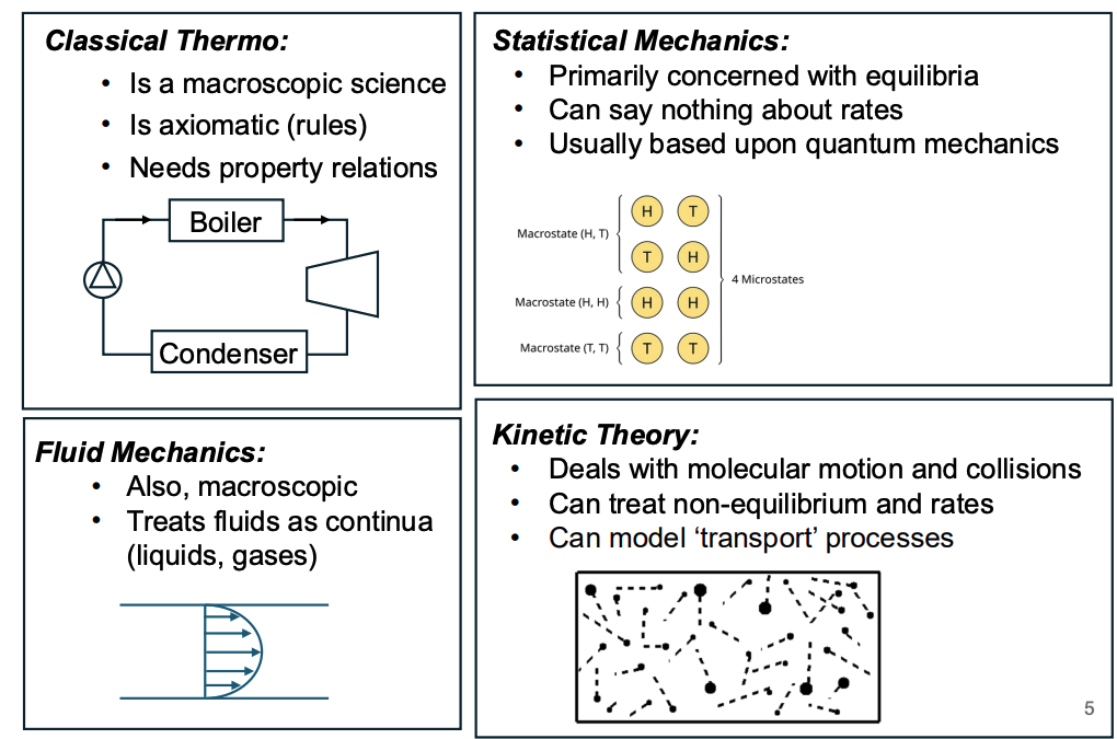
Map of statistical mechanics

Classical thermo

• Macroscopic, looks at bulk properties like temperature pressure

• Based on axioms (rules) and relates properties together

Fluid mech

• Treats system as a continiu

Stat mech

• Concerned about equilibrium not kinetics

• Based off macrostates and microstates, using quantum mechanics to define these states

Kinetic theory

• Deals with mechanical motion and collisions (not bulk)

• Model rates

Intermolecular forces

Our repulsive forces are generally very strong and short ranged. Our attractive forces are generally longer ranged and depend on electron configuration.

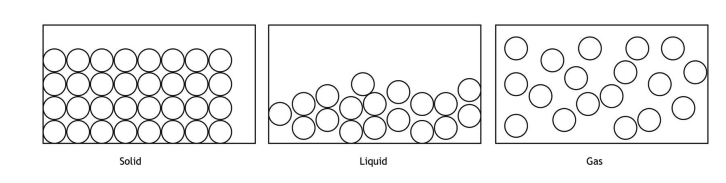
Liquids

• Our molecules are very close together an always interacting, very difficult to model with kinetic theory

Low pressure gases (ideal gas model)

• Molecules are dilute

• Forces important only during collisions and we can ignore intermolecular potential energy

Model for intermolecular forces

We have three models for intermolecular forces

• Hard sphere model (this is what we use to derive the ideal gas equation)

• Sutherland model, this adds attraction (often used to calculate viscosity in gasses)

• Lennard-jones model this adds both attraction and a realistic repulsion model. Results in a potential well where molecules are most stable.
  

the Lennard jones potential : \phi(r) = 4\epsilon \left[ \left( \frac{\sigma}{r} \right)^{12} - \left( \frac{\sigma}{r} \right)^6 \right]
We can define the following quantities:

σ: this is the distance at which the particle energy equals the infinity energy (no energy interaction)

r_e : this is where the particle is in equilibrium, particles are most stable here

r_s : this is the distance of maximum attraction between particles we can assume particles become non interacting ≈ 2.5σ
ε : this is potential well depth so if KT > ε, my particles begin to escape

Velocity distribution function

Definitions

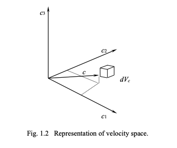
We can describe a velocity distribution function.

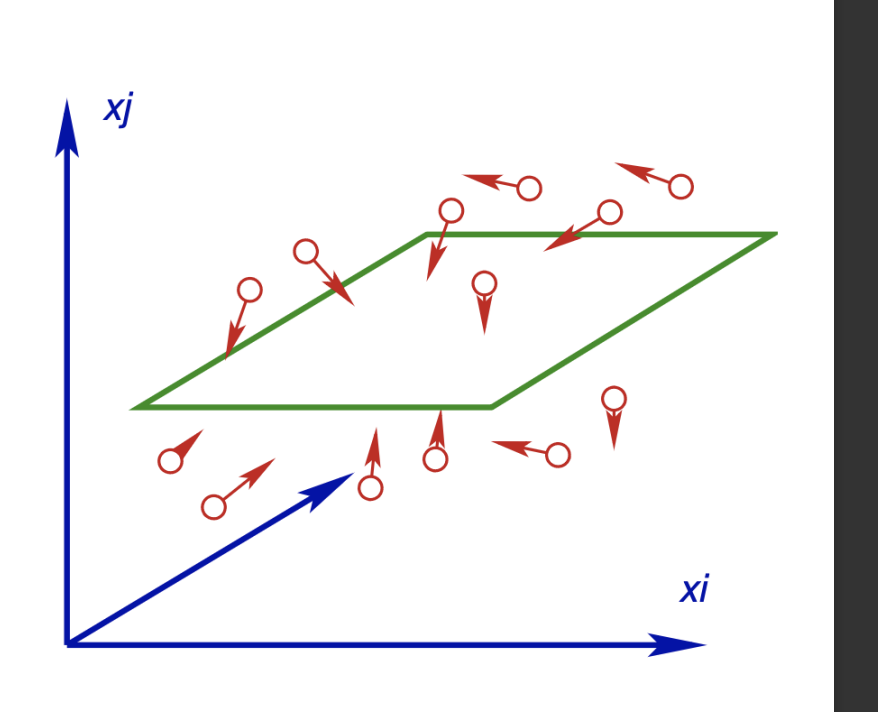
• We use use a cartesian system (x₁, x₂, x₃)

• the number density of molecules is n (number per unit volume)

• the absolute velocity of the particles is (c₁, c₂, c₃ )

speed of particles

this is \sqrt{c_1^2 + c_2^2 + c_3^2}

distribution function

We can define a molecular distribution function as
Average\space no\space of\space class\space c_i\space molecules\space per \space unit \space volume = fdc_1dc_2dc_3 = fdV_c

• If the gas is in equilibrium f = f(c_1, c_2, c_3)

• if the gas is steady but spatially non uniform f = f(c_1, c_2, c_3, x_1, x_2, x_3)

• if non steady f=f(c_1,c_2,c_3,x_1,x_2,x_3,t)

We must normalise this distribution function with the condition that we know the sum of all particles of all classes is a equal to the number density of particles

\int_{-\infty}^{\infty} \int_{-\infty}^{\infty} \int_{-\infty}^{\infty} f(c_i, x_i, t) \, dc_1 dc_2 dc_3 = \int_{-\infty}^{\infty} f \, dV_c = n(x_i, t)

bulk vs peculiar velocity

we can define a BULK (average gas flow velocity) and peculiar velocity (velocity relative to said flow)

C_i = c_i - u_i (Cᵢ is the peculiar velocity)

Ideal gas derivation example

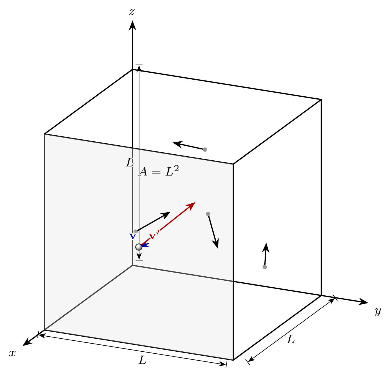
Here we’re considering a box with length L with volume L³ with N particles all with mass m.

momentum change per collision

• Assuming an elastic instantaneous collection with the edge of the box

Particles are moving at speed c₁, and because they bounce back

\Delta p = 2mc_1

rate of collisions

• The force is the total change in momentum over the average time taken to hit.

• The average time it takes the particle to hit the wall is 2L/c_1

So our force per molecule is: F_{molecule}=\frac{m c_1^2}{L}

Total force is F_{total}=\frac{N m \overline{c_1^2}}{L}

pressure:

our pressure is force by unit area L² so:

p=\frac{N m \overline{c_1^2}}{L^3}=\frac{N m \overline{c_1^2}}{V}

symmetry and energy

finally to get to the ideal gas relation we need to relate mc₁² to our temperature.

• Our total kinetic energy T=\frac{1}{2}nm\left(\overline{c}_1^2+\overline{c}_2^2+\overline{c}_3^2\right)=\frac32nkT

• As our three axes are identical we can rewrite this as

T=\frac32nm\left(\overline{c}_1^2\right)=\frac32nkT^{}

so nm\left(\overline{c}_1^2\right)=nkT^{}

final equation

p=\frac{nkT}{V} this is our ideal gas equation where nk = mR

Central goal of kinetic theory

The primary goal of kinetic theory is to find the velocity distribution function f, in terms of our velocities, positions and time.

• We can then evaluate our macroscopic relations from this

Equilibrium velocity and speed distribution

For a gas at equilibrium with no bulk velocity (or if we switch reference frames) AND where f does not vary in space or time. We can simplify our equations:

• No preferred directions, c1 c2 and c3 and identical

• So dependence on speed

• we write this as f_e(C)

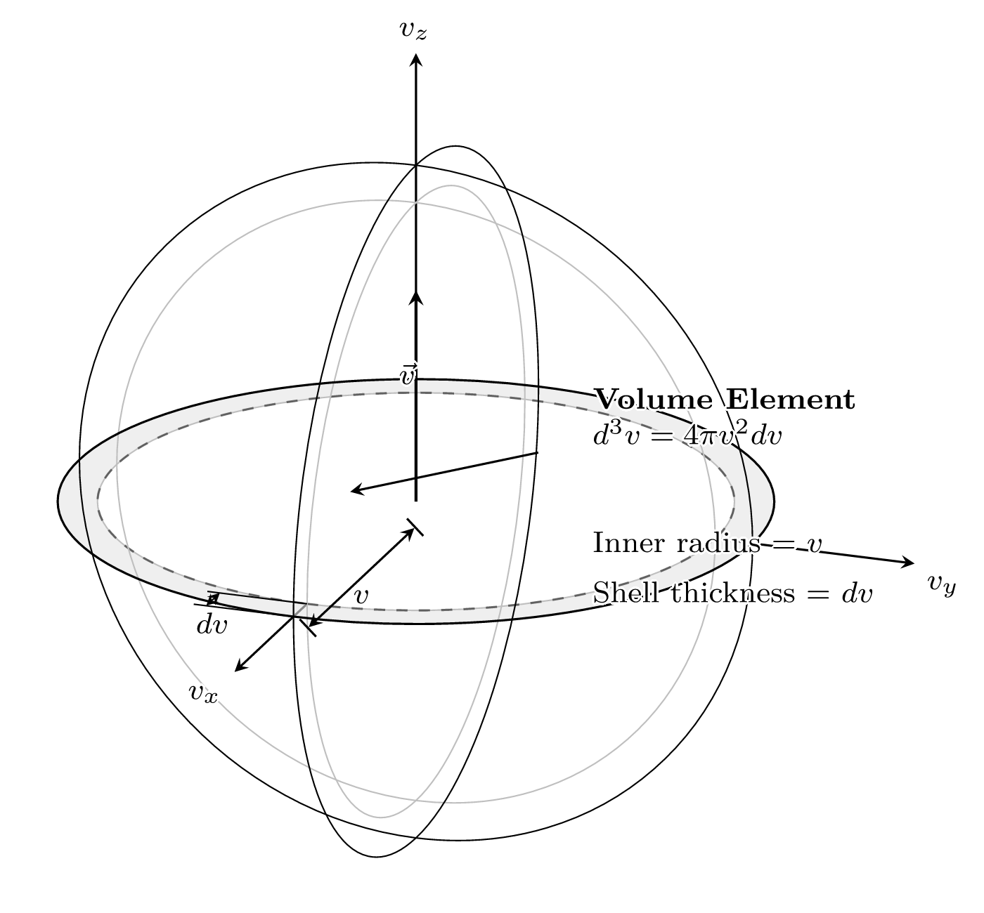
speed distribution function

we can define a speed distribution function g_e(C)

• Because a spherical shell in the velocity space is identical in speed, we define our speed distribution function as

g_e(C) = 4\pi C^2 f_e(C)

normalisation

again if we integrate over all speeds:

\int_{0}^{\infty} g_e \, dC = n

Averages of molecular quantities

Often we want to take averages of molecular quantities

• This is sort of our bridge to the macroscopic qorld.

defining Q

Let Q = Q(c_i) be a quantity which is a function of our molecular velocity

• This can be temperature, pressure energy etc

average

We can thus take a weighted average with the distribution function (remember f is basically our frequency distribution function)

\overline{Q} = \overline{Q}(x_i, t) = \frac{1}{n(x_i, t)} \int_{-\infty}^{\infty} Q(c_i) f(c_i, x_i, t) \, dV_c

Equilibrium simplification

if our gas in equilibrium with no bulk velocity, then we can do:

\overline{Q} = \frac{1}{n} \int_{-\infty}^{\infty} Q(c_i) f(c_i) \, dV_c (still a triple integral)

if q only depends on speed this is even simpler as we can integrate over all speeds instead of all volumes V

\overline{Q} = \frac{1}{n} \int_{0}^{\infty} Q(C) g_e(C) \, dC

Flux of molecules to a surface

We are often interested in the flux (sort of flow rate of molecules through a surface)

• Continuum mechanics models with net flux (momentum flux, heat flux)

• we care about the overall picture not the minutia of particle movement.

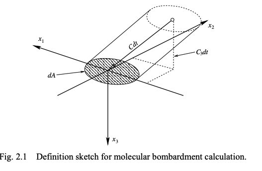
derivation

We will consider a slant cylinder (angled to align with the velocity vector)

• For flux we only care about the component normal to the surface C₃

so:
\text{Number of } C_i \text{ molecules incident on area } dA \text{ in time } dt = C_3 f \, dV_c \, dA \, dt

flux per unit area

\text{Number of } C_i \text{ molecules incident per unit area/time} = C_3 f \, dV_c

total one sided flux (F_+)

• this is defined as particles moving towards a surface so C₃ is +ve

F_+ = \int_{0}^{\infty} \int_{-\infty}^{\infty} \int_{-\infty}^{\infty} C_3 f(C_1, C_2, C_3) \, dC_1 dC_2 dC_3

Flux example (spherical coordinate).

Here we’re doing an example if the gas is in equilibrium with NO bulk velocity.

Trying to work out the one sided molecular flux through a surface.

integrating up F_+ = \int_{0}^{\infty} \int_{-\infty}^{\infty} \int_{-\infty}^{\infty} C_3 f(C_1, C_2, C_3) \, dC_1 dC_2 dC_3

transforming in velocity space

Here if we transform into velocity space, our velocities are spherically symmetric.

To find the flux we need to first work out the vertical velocity.

• This is: C_3 = C \cos\theta

• our velocity volume element is dV_c = C^2 \sin\theta \, dC \, d\theta \, d\phi

  • This has polar angle θ from 0 to \pi/2 (lattitude)

  • Azimuthal angle φ from 0 to 2π

working out integral

F_{e+} = \int_{0}^{2\pi} \int_{0}^{\pi/2} \int_{0}^{\infty} (C \cos\theta) f_e(C) (C^2 \sin\theta \, dC \, d\theta \, d\phi) (all our elements are independent so)

F_{e+} = \left[ \int_{0}^{2\pi} d\phi \right] \left[ \int_{0}^{\pi/2} \sin\theta \cos\theta \, d\theta \right] \left[ \int_{0}^{\infty} C^3 f_e(C) \, dC \right]

result

F_{e+} = (2\pi) \cdot \left( \frac{1}{2} \right) \cdot \left( \frac{n \bar{C}}{4\pi} \right) = \frac{n \bar{C}}{4}

This is a key result that the number of molecules hitting one-quarter of a surface of the number density and mean speed

Later we will show \overline{C}=(\frac{8kT}{\pi m})^{\frac{1}{2}}

Combining this together we get

F_{e+} = \frac{p}{\sqrt{2\pi mkT}}

This is same as ideal gas law

Flux of molecular properties

If we’re interested in the flux of a molecular property Q, like pressure. We can just take a weighted integral

Front face flux: C_3 > 0

F_{Q+} = \int_{0}^{\infty} \int_{-\infty}^{\infty} \int_{-\infty}^{\infty} Q C_3 f \, dV_c

Back face flux: C_3 < 0

F_{Q-} = \int_{-\infty}^{0} \int_{-\infty}^{\infty} \int_{-\infty}^{\infty} Q C_3 f \, dV_c

Flux of molecular properties (pressure)

For some functions we don’t need to use know the exact form of f, because we can define the flux in terms of statistical moments.

To find pressure, we’re going to do a control volume momentum balance, working out the momentum flux first.

Momentum flux (normal)

Incident momentum flux = -\int_{-\infty}^{0} \int_{-\infty}^{\infty} \int_{-\infty}^{\infty} (mC_3) C_3 f(C_i) \, dC_1 dC_2 dC_3

Reflected momentum flux = +\int_{0}^{\infty} \int_{-\infty}^{\infty} \int_{-\infty}^{\infty} (mC_3) C_3 f(C_i) \, dC_1 dC_2 dC_3

Momentum balance

Our total rate of normal momentum loss per unit area equates to the normal stress

• This is basically what we did in ideal gas to find pressure

\sigma_{33} = -\int_{-\infty}^{\infty} \int_{-\infty}^{\infty} \int_{-\infty}^{\infty} (mC_3)C_3 f(C_1, C_2, C_3) \, dC_1 dC_2 dC_3 = -nm\overline{C_3^2}

• We can take out the m and define this as the average of C₃²

Just like in ideal gas because there is no preferred direction:

\overline{C_1^2} = \overline{C_2^2} = \overline{C_3^2} = \frac{\overline{C^2}}{3}

result

So we can get our pressure equation as:

p = \frac{nm\overline{C^2}}{3} = \frac{\rho\overline{C^2}}{3}

pressure energy relation

We can relate this to translational KE as this E_{trans} = \int_{-\infty}^{\infty} \frac{mC^2}{2} f \, dV_c = \frac{\rho\overline{C^2}}{2}

so we get the result: p = \frac{2}{3}E_{trans}

non-equilibrum result

In a non equilibrium, we have an addition “left over term”

• Our wall stress is not exactly equal to our pressure. So:

\tau_{33} = \sigma_{33} - (-p) = -\rho \overline{C_3 C_3} + \frac{\rho(\overline{C_1 C_1 + C_2 C_2 + C_3 C_3})}{3}

• Viscous normal stresses are normally tiny so we ignore them

Defining temperature

definition of kinetic temperature

can define temperature with kinetic theory, it is defined as being proportional to the mean translational ke of a molecule

• Temperature is a macroscopic quantity and not defined for single molecules.

\frac{3}{2} k T_K = \frac{m \overline{C^2}}{2}

scaling to macroscopic properties

Remember that we can define our pressure as:

\frac{3}{2} \rho R T_K = E_{trans}

Subbing this together we arrive at the ideal gas law.
p = \rho R T_K

Kinetic vs thermodynamic temperature
There is a distinction between kinetic temperature which is defined in terms of our kinetic energy, and our thermodynamic equation which is defined by our ideal gas law.

For general applications these are identical, so T_K = T_A = T, as we can link both with ideal gas law.

• However thermodynamics only deals with systems in equilibrium, so thermodynamic temperature is not always defined

• Kinetic theory by contrast will always define a temperature, as the mean kinetic energy of a molecule is always an easily defined quantity

Energy of monatomic, diatomic and polyatomic molecules

The structure of a molecule affects how much energy it can store

Relationship between degrees of freedom and specific energy

For each degree of freedom of motion, we can assign an energy. So that the total energy per unit mass is:
e = F\frac{RT}{2}

Monoatomic

These can store E=E_{trans}=\frac{nm\overline{C^{2}}}{2}=\frac{3}{2}\rho\overline{R}T

• the specific energy per unit mass is e = \frac{3}{2}RT

• This is because they only have three degrees of freedom, x,y and z

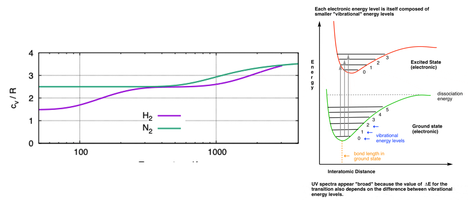
Diatomic molecules

• These still have the 3 degrees of freedom from x,y,z

• But there are additional vibration and rotation modes too.

• There are two rotation modes, for basically the primary moments of inertia, the length wise moment basically stores no energy

• There are two vibration modes, this is for both the energy stored in the bond and kinetic energy of vibration

Poly atomic molecules

These are much more complicated, generally with three degrees of rotation, but their vibrational modes are too complicated to simply break down.

note on internal energy

• In classical thermo, energy is split into kinetic energy, gpe and internal energy which consists of intermolecular potential energy as well as molecular mode energy

• Kinetic theory, internal energy refers to ONLY the molecular mode energy

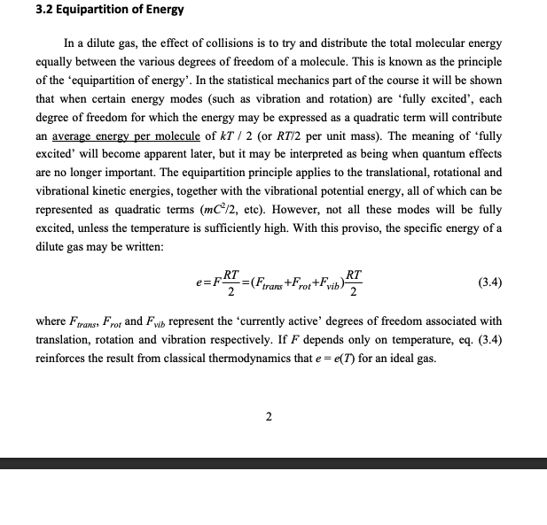
Equipartition of energy.

The concept here is basically a gas will try distribute molecular energy equally between all its modes and degrees of freedom. This is known as the Equipartion of Energy\

• We will see from stat mech that every DOF that can be expressed as a quadratic term (like mC²/2) will result in an average energy per molecule of kT/2 or RT/T (per unit mass)

• e = F\frac{RT}{2} = (F_{trans} + F_{rot} + F_{vib})\frac{RT}{2}

However not every mode will be excited at every temperature

Predicting specific heat capacity

We can predict the specific heat capacity from the
Our energy is e = F\frac{RT}{2} = (F_{trans} + F_{rot} + F_{vib})\frac{RT}{2}

Specific heat capacity is defined as change in energy per unit temp (at constant volume)

differentiating our energy equation we get:

c_v = \left( \frac{\partial e}{\partial T} \right)_v = (F_{trans} + F_{rot} + F_{vib}) \frac{R}{2}

However, our modes are only excited at different temperature:

• Our translational modes are always active, so minimum cᵥ of 1.5

• Because of quantum mechanics our vibrational modes and rotation modes are quantised and only activated above certain temperatures

• Above around 10K our two rotation modes are unlocked (hydrogen has a tiny moment of inertia so is special)

• Our two vibration modes are typically only active at thousands of degrees

Predicting specific heat ratio

For an ideal gas our heat capacities are related by c_p - c_v = R

We are often interested in our specific heat ratio γ as it is important in isotropic processes

This is defined as \gamma = \frac{c_p}{c_v} = \frac{F + 2}{F}

For monotonic cases we are predicting a ratio of 1.67 which lines up very well

For diatomic we are predicting from 1.42 to 1.28 at high temperatures

• This matches well for air which is at 1.4

The more degrees of freedom the closer γ gets to approaching one

Deriving maxwell boltzmann distribution

This is an attempt at solving for a velocity distribution function f in terms of C₁, C₂, and C₃

• This is very difficult for a non-equilibrium gas

• But comparatively easy for an equilibrium gas (no bulk velocities or temperature gradients)

• Maxwell introduced a further assumption of statistical independence of the three axes (this turns out to be true but unjustified)

  • mathematically this is f_e(C_i) = n \times \psi_1(C_1) \times \psi_2(C_2) \times \psi_3(C_3)

  • ψ is the distribution function for each axis

Example: using Maxwell assumption, find molecular velocity and speed distributions

Starting from f_e(C_i) = n \times \psi_1(C_1) \times \psi_2(C_2) \times \psi_3(C_3)

Then we can take the log:

\ln f_e = \ln n + \ln \psi_1 + \ln \psi_2 + \ln \psi_3

Now taking the gradient of this:

\nabla_C(\ln f) = \frac{1}{f_e} \begin{bmatrix} \frac{\partial f_e}{\partial C_1} \\ \frac{\partial f_e}{\partial C_2} \\ \frac{\partial f_e}{\partial C_3} \end{bmatrix} = \begin{bmatrix} \frac{1}{\psi_1} \frac{\partial \psi_1}{\partial C_1} \\ \frac{1}{\psi_2} \frac{\partial \psi_2}{\partial C_2} \\ \frac{1}{\psi_3} \frac{\partial \psi_3}{\partial C_3} \end{bmatrix}

And because we also know that f_e = \phi(C_1^2 + C_2^2 + C_3^2)

We now have the differential equation (for each axes)

• First equation: \frac{1}{\psi_i}\frac{\partial\psi_i}{\partial C_i}=\frac{1}{f_{e}}\frac{\partial f_{e}}{\partial C_{i}}

• From chain rule of the spherical symmetric:

  • \frac{\partial}{\partial C_1} \phi(C^2) = \phi'(C^2) \cdot 2C_1

• We get this after combining \frac{1}{\psi_1} \frac{d\psi_1}{dC_1} = 2 C_1 \cdot \phi'(C^2)

  • \phi^{\prime}(C^2) must be constant, as our LHS only depends on C₁ not C₂ or C₃

so we get \frac{1}{\psi_i} \frac{\partial \psi_i}{\partial C_i} + \beta C_i = 0

solution for differential equation

this has the solution from separation of variables of:

\psi_i = \alpha_i \exp\left(-\frac{\beta C_i^2}{2}\right)

combining for velocity distribution

now we can recombine as f_e(C_i) = n \times \psi_1(C_1) \times \psi_2(C_2) \times \psi_3(C_3)

so f_e = n \alpha_1 \alpha_2 \alpha_3 \exp\left(-\beta \frac{C_1^2 + C_2^2 + C_3^2}{2}\right)

speed distribution

We can also find our speed distribution using the previous relationship (derived from spherical shell)

g_e(C) = 4\pi C^2 f_e(C)

g_e = 4\pi C^2 \alpha \exp \left( -\frac{\beta C^2}{2} \right)

finding boundary conditions

To find our boundary conditions α and β:

• α can be found by normalisation since \int_{0}^{\infty} g_e(C) dC = n

• β is found with kinetic energy since \frac{1}{n} \int_{0}^{\infty} \frac{1}{2}mC^2 g_e(C) \, dC = \frac{3}{2}kT

• Use data book integral tables

Maxwell boltzmann velocity and speed distribution

Our expressions are thus:

f_e(C) = \frac{n}{(2\pi RT)^{3/2}} \exp\left(-\frac{C^2}{2RT}\right) (this is just a normalised gaussian)

g_e(C) = 4\pi C^2 \frac{n}{(2\pi RT)^{3/2}} \exp\left(-\frac{C^2}{2RT}\right)

‘

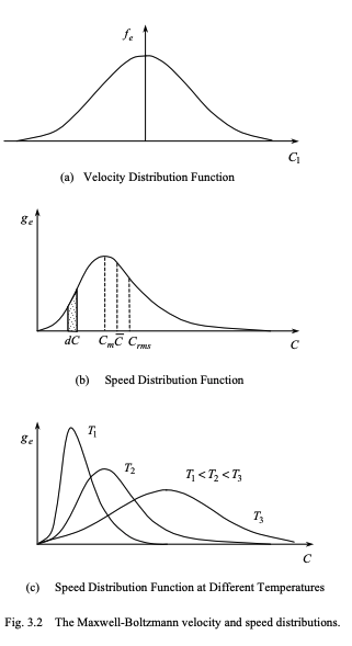
Characteristics of maxwell boltzmann distribution

Our maxwell boltzmann functions are:
f_e(C) = \frac{n}{(2\pi RT)^{3/2}} \exp\left(-\frac{C^2}{2RT}\right) (this is just a normalised gaussian)

g_e(C) = 4\pi C^2 \frac{n}{(2\pi RT)^{3/2}} \exp\left(-\frac{C^2}{2RT}\right)

We can define three speeds.

• C_m = \sqrt{2RT} this is the mode speed

• \overline{C} = \sqrt{\frac{8RT}{\pi}} mean molecular speed

• C_{rms} = \sqrt{\overline{C^2}} = \sqrt{3RT} this is the rms speed

Sometimes we are interested in finding what fraction of molecules are above a certain speed/energy

• EG for kinetics

• We can solve for this using an error function (defined as the normalised integral of a gaussian)

eg:

I = \frac{1}{n} \int_{C_0}^{\infty} g_e(C) \, dC = 1 - \frac{1}{n} \int_{0}^{C_0} g_e(C) \, dC = 1 - \int_{0}^{C_0} \frac{4\pi C^2}{(2\pi RT)^{3/2}} \exp\left(-\frac{C^2}{2RT}\right) \, dC

We can simplify this by using the substitution \xi = C/\sqrt{2RT}

I = 1 - \frac{4}{\sqrt{\pi}} \int_{0}^{\xi_0} \xi^2 \exp(-\xi^2) \, d\xi

integrating by parts we get:

I = 1 + \frac{2\xi_0 \exp(-\xi_0^2)}{\sqrt{\pi}} - erf(\xi_0)

Departures from equilibrium in kinetic theory

So far we have only considered gasses in equilibrium, this discusses how collisions are used to restore equilibrium.

Dynamic nature of equilibrium

• For gases in equilibrium, collisions are required to maintain the equilibrium

• At the molecular state collisions are obviously a dynamic process

• Change in classes however for each collision that changes a molecule from velocity class Cᵢ to Cᵢ’

• Inverse collisions it is a statistically certainty (due to large numbers) that a similar inverse collision will result in another molecule changing from velocity class Zᵢ’ to Zᵢ

• as such equilibrium is maintained.

hierachy of relaxation

If a gas is perturbed from equilibrium, and the perturbation is released, molecular collisions will act to restore the equilibrium.

However the speed of restoration and the “relaxation time” will vary depending on mode.

Mode	Relaxation Time / Collisions	Key Detail
Translational	Very Short (~few collisions)	Molecules quickly redistribute "zoom" speeds.
Rotational	Very Short	Spinning modes balance almost as fast as translation.
Vibrational	Much Longer	"Wiggling" modes can take many more collisions to balance, which is a major factor in hypersonics.
Chemical	Longest (Orders of magnitude more)	Reaching chemical balance requires the most collisions. But velocity distribution is locally maxwellian

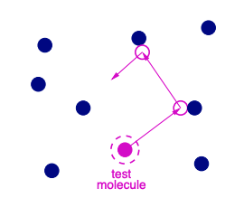
Considering a test molecule and mean free path

Simplified test molecule model

To analyse how frequency collisions are in a gas we will analyse a simplified model:

Here we will consider a “test” molecule moving a speed c with all particles at rest

• We want to find expression for the collisions per unit time (collision frequency)

• Average distance between collisions (mean free path)

• Overall molecular collision rate in the gas (number of collisions in a volume gas)

finding collisions per unit time

Basically all we’re doing here is considering the Volume swept out by our test particle, and seeing density of particles

• Volume swept out by test particle per unit time: \pi d^2 \bar c

• No of particles per unit volume is: n

• Hence our frequency is \tau = n \pi d^2 \bar c

finding mean free path

our speed is c, and we can write this in the form \bar c = \lambda \tau

• Our mean free path λ is thus:

\frac{1}{nπd²}

total collision rate

this is our collision frequency multiplied by the number of particles

• We need to divide by 2 as each collision occurs between 2 particles.

Z = \frac{n\tau}{2} = \frac{n²πd²\bar c}{2}

Real model

If we were considered that multiple particles are moving, not just our test particle we have a factor of √2, Our real expressions are:

• Total Collision Rate (Z): Z = \frac{\sqrt{2} \pi n^2 d^2 \overline{C}}{2} = \frac{\sqrt{2} \pi n^2 d^2}{2} \sqrt{\frac{8kT}{\pi m}}

• Mean free path (λ): \lambda = \frac{1}{\sqrt{2} \pi n d^2}

It’s quite typical in kinetic theory for simple analysis to result in the right form but wrong coefficients.

Extending collision rate to mixtures

For mixtures we can treat this as two “self” terms and also a “coupling” term

self terms

• Z_{AA} = \frac{\sqrt{2} \pi n_A^2 d_A^2 \overline{C}_A}{2} = \frac{\sqrt{2} \pi n_A^2 d_A^2}{2} \sqrt{\frac{8kT}{\pi m_A}}

• Z_{BB} = \frac{\sqrt{2} \pi n_B^2 d_B^2 \overline{C}_B}{2} = \frac{\sqrt{2} \pi n_B^2 d_B^2}{2} \sqrt{\frac{8kT}{\pi m_B}}

unlike (coupling term

Here our relationship is a bit different:

• Z_{AB} = \sqrt{2} \pi n_A n_B d_{AB}^2 \sqrt{\frac{4kT}{\pi m_{AB}}}

d_{AB} = (d_A + d_B) / 2 we have this as the average diameter

m_{AB} = \frac{m_A m_B}{m_A + m_B} we also have the reduced mass, common to reduce 2 body systems to 1 body

Chemical reaction rates

why it is difficult to predict rates

It is very difficult to predict chemical reaction rates due to the shear number of avenues that a given reaction can take place.

A reaction like H_2 + I_2 \rightarrow 2HI does occur via hydrogen + iodine collision and is relatively simple

But a reaction like H_2 + Br_2 = 2HBr takes place through 5 elementary processes

\begin{aligned} Br_2 + M &\rightarrow 2Br + M \\ Br + H_2 &\rightarrow HBr + H \\ H + Br_2 &\rightarrow HBr + Br \\ HBr + H &\rightarrow Br + H_2 \\ 2Br + M &\rightarrow Br_2 + M \end{aligned}

modelling rates

Only considering simple bimolecular reactions, three things generally need to happen fo a reaction.

• The Collision: The molecules must actually hit each other (this is the Z_{AB} rate we discussed earlier).

• The Energy Barrier: They must hit with enough "punch." Specifically, the kinetic energy along their line of centers must exceed the activation energy (\epsilon_0).

• The Orientation (Steric Factor): They must hit at the right angle. If they hit "sideways," the bonds might not break even if they have enough energy.

This results in the equation

\begin{pmatrix} \text{Rate of} \\ \text{reacting} \\ \text{collisions} \end{pmatrix} = \begin{pmatrix} \text{Rate of} \\ \text{collisions} \end{pmatrix} \times \begin{pmatrix} \text{Fraction of} \\ \text{collisions with} \\ \text{sufficient energy} \end{pmatrix} \times \begin{pmatrix} \text{Fraction of sufficiently} \\ \text{energetic collisions that} \\ \text{result in a reaction} \end{pmatrix}

Combining our factors:

• First term is from our Z ab collision rate

• Second term is from maxwell boltzmann distribution

• Third term is steric factor (found emperically or via QM)

\text{Rate} = n_A n_B f(T) T^{1/2} \exp\left(-\frac{\epsilon_0}{kT}\right) = k_f(T) n_A n_B

Arhenius equation

many experiments for kf (the forward rate constant) are well fitted by:

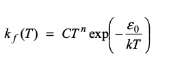
k_f(T) = CT^n \exp \left( -\frac{\epsilon_0}{kT} \right)

The exponential term is very well predicted by kinetic theory, which was first introduced as a empirical factor by ahrenius

• However still need to empirically prescribe factors for steric factor and activation energy.

Law of mass action

If we consider a bimolecular iodine hydrogen equation. From the previous rate equations, we know that:

\text{Forward Rate} = k_f(T) n_{H_2} n_{I_2} (H₂ + I₂ → 2HI)

\text{Backward Rate} = k_b(T) n_{HI}^2 (2HI → H₂ + I₂ )

if the mixture is in equilibrium then
k_f(T) n_{H_2} n_{I_2} = k_b(T) n_{HI}^2 \implies \frac{n_{HI}^2}{n_{H_2} n_{I_2}} = \frac{k_f(T)}{k_b(T)}

or in terms of partial pressures as well as we know p = nkT (where kT is same for both gasses)

\frac{n_{HI}^2}{n_{H_2} n_{I_2}} = \frac{p_{HI}^2}{p_{H_2} p_{I_2}} = \frac{k_f(T)}{k_b(T)} = K_p(T)

This is the law of mass action, because our equilibrium point depends on the concentration of our reactants

Translational and rotational non-equilibrium

Viscous stresses and heat conduction are the macroscopic result of local departures from the maxwellian equilibrium.

It is quite difficult to seriously disturb the maxwellian distribution and in real macroscopic situations this is generally confined to just

• Boundary layers (very high velocity gradients and thus viscosity)

• Shockwaves (very high temperature gradients and thus conduction)

Generally we can almost ignore viscosity and heat conduction in gases outside of these regions as the molecular velocity distribution is in equilibrium and near maxwellian.

Origins of viscous stress.

Viscous stress is ultimately caused by momentum being carried across layers

Molecular definition of stress

• Normal stress this is when the momentum direction and the momentum transport direction are the same

• Shear stress this is when the momentum direction and momentum transport direction are orthogonal.

governing equation

Our shear stress, this coupling term is given by the covariance of our stress terms.

\sigma_{ij} = -\int_{-\infty}^{\infty}\int_{-\infty}^{\infty}\int_{-\infty}^{\infty} mC_i C_j f(C_1, C_2, C_3) \, dC_1 dC_2 dC_3

\sigma_{ij} = -\rho \overline{C_i C_j}

• Basically a velocity covariance, physically this is a measure of how our velocity depends on different layers

• Looks very similar to our turbulent stress forms in 3A1 boundary layers

Once we know our velocity distribution function, we would be able to directly evaluate our shear stress

• Our maxwellian velocity equation is symmetric, so results in no shear stress

• Can find an exact model by solving the “Boltzmann equation” but this is very complicated

• We will use a simple mean free path model

Mean free path model of shear stresses

We will use a simple mean free path model to try solve for how our viscosity varies.

setup

• We will consider a layer of fluid where the horizontal velocity varies with the vertical direction.

• Considering a thin plane of interest, our bulk velocity (which is only in the x₁ direction) is : u(x_2) \cong u(0) + x_2 \frac{du}{dx_2}

• Ontop of this bulk velocity we will superpose our peculiar velocities

Velocity is : (u + C₁, C₂, C₃)

Considering flux between layers

We will remember for steady state (random) molecules, the molecular flux through a given plane is \frac{\rho \bar C}{4} (per unit area)

• We can use this even though our flow isn’t completely random, because the bulk velocity is parallel to the plane.

Now if we consider the momentums:

• \text{Flux of } x_1\text{-momentum from below} \cong \frac{\rho \overline{C}}{4} \left[ u(0) - \lambda \frac{du}{dx_2} \right]

• \text{Flux of } x_1\text{-momentum from above} \cong \frac{\rho \overline{C}}{4} \left[ u(0) + \lambda \frac{du}{dx_2} \right]

The change in momentum is our shear stress

\sigma_{12} = \tau_{12} \cong \frac{\rho \overline{C} \lambda}{2} \frac{du}{dx_2}

As we define a dynamic viscosity from newton’s law of viscosity \tau_{12} = \mu du/dx_2

we can define the dynamic viscosity with this simple model as

\mu=\frac{\rho\overline{C} \lambda}{2}=\frac{1}{d^2}\sqrt{\frac{mkT}{\pi^3}}

• Viscosity only depends on temperature and type of molecule (mass and diameter)

• The more complex chapman enskog theory that solves the boltzman equation gives \mu = \frac{5\pi}{32} \rho \overline{C} \lambda \approx 0.491 \rho \overline{C} \lambda

• our simple model is remarkably close

Effect of intermolecular forces on viscosity

In reality our viscosity doesn’t scale with √T, it scales faster than √T. This is due to the effects of intermolecular forces.

• We can improve this by using the Sutherland model of intermolecular forces (which models molecular attractions)

Here we’re basically saying the intermolecular forces increases the effective diameter of the molecule

• At low temperatures the effective diameter is large, but at high temperatures the effective diameter is smaller, this results in the viscosity dropping faster than expected.

• From before \mu=\frac{1}{d_{eff}^2}\sqrt{\frac{mkT}{\pi^3}}

Our sutherland model gives us the approximation:

\frac{\mu}{\mu_0}=\left(\frac{T}{T_0}\right)^{1/2}\frac{1 + A/T_0}{1 + A/T}

• we have a scaling factor at different temperatures now

• A is the sutherland constant which is a gas constant.

Modelling heat conduction with mean free path model

We can use a similar model to viscosity to model heat conduction. For heat conduction we’re basically replacing our momentum transport between layers with kinetic energy between layers.

Our transport equation is (with a Q = mC^2/2 instead of momentum)

q_{j}=\int_{-\infty}^{\infty}\int_{-\infty}^{\infty}\int_{-\infty}^{\infty}\frac{1}{2}mC^2C_{j}f(C_1,C_2,C_3)\,dC_1dC_2dC_3

q_j = \frac{\rho \overline{C^2 C_j}}{2} (more compact)

So this can be rewritten as

This is only valid in monatomic gases where energy is carried by translational kinetic energy

energy fluxes

Again using the same random molecule flux equation across a boundary

• Upward flux: q_2^+ = \frac{n \bar{C}}{4} m c_v \left\{ T_0 - \lambda \frac{dT}{dx_2} \right\}

• Downward flux: q_2^- = \frac{n \bar{C}}{4} m c_v \left( T_0 + \lambda \frac{dT}{dx_2} \right)

• net upward flux: q_2 = q_2^+ - q_2^- = -\frac{\rho \bar{C}}{2} \lambda c_v \frac{dT}{dx_2}

  • q_2 = \underbrace{\left( \frac{1}{4} \rho \bar{C} \right)}_{\text{Mass Flux}} \times \underbrace{\left( -2 \lambda c_v \frac{dT}{dx_2} \right)}_{\text{Energy Difference}}

results:

comparing this with fourier’s law of heat conduction:

\text{cf. } q_2 = -k \frac{dT}{dx_2} \implies k = \frac{\rho \bar{C} \lambda c_v}{2}

This is quite a bit worse than chapman-enskog (solving boltzmann) which gives:

k = \frac{\rho \overline{C} \lambda \beta c_v}{2} = \frac{\beta c_v}{d^2} \sqrt{\frac{mkT}{\pi^3}} \quad \left( \beta = \frac{5}{2} \right)

We are off by a factor of 2.5

• This is because we’re neglecting the fact that more energetic molecules come from further away

extending to polyatomic molecules

• We can extend the chapman-enskog result to poly atomic molecules

• We are assuming that the velocity correlation (energetic molecules from further away) is only relevant for translational modes. So we can replace \beta c_v with:

  • \beta \frac{3R}{2} + \left( c_v - \frac{3R}{2} \right)

our expression is thus:

k = \frac{\rho \bar{C} \lambda}{2} \left[ \beta \frac{3R}{2} + \left( c_v - \frac{3R}{2} \right) \right] \quad \left( \beta = \frac{5}{2} \right)

Prandtl number from kinetic theory

This is the ratio of our momentum diffusion to our heat diffusion.

Pr=\frac{\mu/\rho}{k/{c_p\rho}}=\frac{c_p\mu}{k}

• We already have kinetic theory expressions for all of these, so we can get an equation:

Pr=\frac{c_p \mu}{k}=\frac{2\gamma}{2 + 3(\beta- 1)(\gamma- 1)}\quad\left(\beta=\frac{5}{2}\right)

This gives quite a good match to our experimental results using the Chapman-Enskog relations, especially for monoatomic and diatomic

Gas	γ	Pr Experimental	Pr Equation (5.9)
Ne (Neon)	1.67	0.66	$0.67
Ar (Argon)	1.67	0.66	0.67
H_2	1.41	0.74	0.73
Air	1.40	0.70	0.74
CO_2	1.31	0.79	0.77
C₂H₆	$1.19$	0.82	0.83
H₂O	1.32	0.87	0.77$$

Diffusion with kinetic theory.

This is our final transport property, instead of momentum or kinetic energy it is the molecular identity which is being moved.

this is governed by fick’s law

j_{A2} = -D_{AB} \frac{d\rho_A}{dx_2}

mean path analysis

For a simple model if we assume our dissimilar molecules are identical, but identical, we can do the exact same analysis with fluxes to show:

D_{AB}=D_{BA}=D=\frac{\bar{C} \lambda}{2}

Chapman-enskog gives us a coefficient of 3\pi/16 instead which is 0.59

schmidt number

We can work out a schmidt number which is a ratio of momentum diffusion to mass diffusion

Sc = \frac{\text{Viscosity}}{\text{Density} \times \text{Diffusion}} = \frac{\mu}{\rho D}

Plugging in our chapman-enskog coefficients we get

Sc \approx 0.85

• this means mass and momentum diffuse at nearly the same rate

Lewis number

We can do a similar thing with heat, with the lewis number. Ratio of thermal diffusivity to mass diffusivity (Sc/Pr)

• This is important in combustion

• if Le ≈ 1 this means heat and fuel molecules are travelling at the same speed, so our flame thickness and reaction zone is similar

• Kinetic theory predicts 1.2, the actual value is closer to 1

what this means

The fact our prandtl, schmidt and lewis numbers are all relatively close to one for many gases allows for simplifications, as we can assume momentum, heat and mass all diffuse at the same rate

The boltzmann equation (intro and derivation)

This is a PDE which derives the evolution of the velocity distribution function

• it is the master equation of gas kinetic theory, analogous to navier stokes (which can be derived from this)

• if it can be solved for a particular molecular model and boundary conditions, then we can fully define a system and work out all the macroscopic properties
  

Derivation of the boltzmann equation

Background:

We will start off looking at a 3d control volume and tracking how the class cᵢ molecules evolve.

• This is due to leaving and entering the control volume (fluxes)

• collisions within the control volume

Rate of increase of class c_i molecules in dV_x = \frac{\partial}{\partial t}(f dV_c dV_x) = \frac{\partial f}{\partial t} dV_c dV_x

Fluxes:

Looking first at just the x1 direction:

• Flux of class cᵢ molecules into LH face: F_1^{-}=C_1fdV_{c}dx_2dx_3\text{ }

• Flux of class cᵢ molecules out of RH face: F_1^+ = F_1^- + \frac{\partial}{\partial x_1} (c_1 f dV_c dx_2 dx_3) dx_1

• Net inflow in x₁ direction: -\frac{\partial}{\partial x_1}(c_1f)dV_{c}dV_{x}

Now we can have inflow from all the directions, so:

• -\left\{\frac{\partial}{\partial x_1}(c_1f)+\frac{\partial}{\partial x_2}(c_2f)+\frac{\partial}{\partial x_3}(c_3f)\right\}dV_{c}dV_{x} Or using vector notation:

• -\nabla\cdot(\mathbf{c}f)dV_{c}dV_{x}

collisions:

now locking at how classes change due to collisions

\left[ \frac{\partial f}{\partial t} \right]_{collisions} dV_e dV_x

combining it all together

Essentially this is:

(\text{Rate of increase of class } c_i \text{ molecules}) = (\text{Net total inflow of class } c_i \text{ molecules}) + (\text{Rate of increase due to collisions}) \left(\frac{\partial f}{\partial t}\right) dV_c dV_x = -\nabla \cdot (\mathbf{c} f) dV_c dV_x + \left[\frac{\partial f}{\partial t}\right]_{\text{collisions}} dV_c dV_x

\frac{\partial f}{\partial t} + \nabla \cdot (\mathbf{c} f) = \left[\frac{\partial f}{\partial t}\right]_{\text{collisions}} now removing the control volume terms

because cᵢ is independent of xᵢ, we’re treating x and c as independent variables in phase space, we can further simplify to

\frac{\partial f}{\partial t}+c\cdot \nabla f=\left[\frac{\partial f}{\partial t}\right]_{\text{collisions}}

Einstein summation notation

This is basically a way of implying summation to avoid writing out lots of summations

repeated subscript rule

• If a subscript appears twice in a term, a summation is implied so:

• in \frac{\partial f}{\partial t} + c_j \frac{\partial f}{\partial x_j} = \left[ \frac{\partial f}{\partial t} \right]_{\text{collisions}}the c_j \frac{\partial f}{\partial x_j} term, this refers to:

• c_1 \frac{\partial f}{\partial x_1} + c_2 \frac{\partial f}{\partial x_2} + c_3 \frac{\partial f}{\partial x_3}

Boltzmann equation (collision term)

character of collisions

Before discussing how to solve the Boltzmann equation, we need to express the collision term in terms of the distribution function and molecular velocity components.

• Restricting the analysis to collisions between two molecules (quite reasonable actually) it is possible to develop expressions for the collision rate.

• We have replenishing collisions and depleting collisions

This leads to this equation

\frac{\partial f}{\partial t} + c_j \frac{\partial f}{\partial x_j} = \left[ \frac{\partial f}{\partial t} \right]_{\text{replenishing}} - \left[ \frac{\partial f}{\partial t} \right]_{\text{depleting}}

mathematical detail

The boltzmann equation is so annoying because these collision terms are defined by integrals

• This is a integro-differential equation, our collision terms involve integrals of our velocity distribution function

molecular models

• it is possible to find analytic solutions for hard-spheres (not very realistic)

• other intermolecular force models need to be numerically solved

Deriving maxwell boltzmann distribution via boltzmann equation

This is one of the few analytic solutions of the maxwell boltzmann equation. Our key simplifying assumptions are:

• Steady state so no spatial or temporal derivatives

• as such our replenishing collisions equal our depleting collisions

• \left[ \frac{\partial f}{\partial t} \right]_{\substack{\text{replenishing} \\ \text{collisions}}} = \left[ \frac{\partial f}{\partial t} \right]_{\substack{\text{depleting} \\ \text{collisions}}}

collision balance

our key principle here is the collision balance, this is basically our original and inverse collisions.

Our collision balance will be satisfied if:

f(c_{i}^{\prime})f(z_{i}^{\prime})=f(c_{i})f(z_{i}) this is basically formalising the idea of collisions and inverse collisions

taking logs

This becomes easier if we take the log:

\ln\{f(c_{i}^{\prime})\}+\ln\{f(z_{i}^{\prime})\}=\ln\{f(c_{i})\}+\ln\{f(z_{i})\}

This tells us that the quantity \ln(f) is conserved during a collision—the total "sum of \ln(f)" for the two molecules is the same before and after they hit.

applying conservation laws

because ln(f) is conserved, we know it must be a linear conservation of my other conserved quantities:

so \ln\{f(c_{i})\}=\underbrace{b\frac{m(c_1^2 + c_2^2 + c_3^2)}{2}}_{\text{Kinetic Energy term}}+\underbrace{a_1mc_1+a_2mc_2+a_3mc_3}_{\text{Momentum terms}}+\text{const}

Now taking inverse logs of this:

\ln\{f(c_i)\} = b \frac{m(c_1^2 + c_2^2 + c_3^2)}{2} + a_1 m c_1 + a_2 m c_2 + a_3 m c_3

applying boundary conditions

now we can solve for the constants a and b, this is via the same number and KE boudnary conditions as before.

This gives:

f(c_1, c_2, c_3) = \frac{n}{(2\pi RT)^{3/2}} \exp \left\{ -\frac{(c_1 - u_1)^2 + (c_2 - u_2)^2 + (c_3 - u_3)^2}{2RT} \right\}

Non equilibrium solutions of boltzmann equation

Apart from the chapman-enskog solutions there are few non equilibrium analytic solutions for the boltzmann equation.

There are two avenues for solving:

Bhatnager-Gross-Krook (BGK)

This is a simplified boltzmann equation from simpifying the collision integrals, also known as the “krooked” boltzmann

\frac{\partial f}{\partial t} + c_j \frac{\partial f}{\partial x_j} = -\frac{(f - f_e)}{\tau}

• This assumes every collision nudges the distribution function back to equilibrium

• Depleting collisions (-f/\tau): This part is fairly accurate; it correctly models molecules leaving their velocity class due to hits

• Replenishing collisions (f_e/\tau): This is the weak link. It assumes that whenever molecules collide and "enter" a new velocity class, they have instantly reached equilibrium. In reality, it takes several collisions for that to happen.

• τ is the time constant between colisions

monte carlo numerical techniques

this is often used for rarefied gas dynamics where NS equation doesn’t apply (when the gas is very thin)

Moments of the Boltzmann equation

Although the solving the boltzmann equation will result in all the information involved in the system, as we know this is generally very difficult

• An alternative method is to take statistical moments of the boltzmann equation:

• Here we’re basically multiplying the boltzmann equation by a quantity of interest and integrating

Example: finding the molecular quantity moment

Our boltzmann equation is:

\frac{\partial f}{\partial t}+c\cdot \nabla f=\left[\frac{\partial f}{\partial t}\right]_{\text{collisions}}

Now taking the moment with a a given molecular quantity Q

\int_{-\infty}^{\infty} Q \frac{\partial f}{\partial t} dV_c + \int_{-\infty}^{\infty} Q c_j \frac{\partial f}{\partial x_j} dV_c = \int_{-\infty}^{\infty} Q \left[ \frac{\partial f}{\partial t} \right]_{\text{COLL.}} dV_c

Pulling out derivatives of the integral
\frac{\partial}{\partial t} \left( \int_{-\infty}^{\infty} Q f dV_c \right) + \frac{\partial}{\partial x_j} \left( \int_{-\infty}^{\infty} Q c_j f dV_c \right) = \int_{-\infty}^{\infty} Q \left( \frac{\partial f}{\partial t} \right)_{\text{coll.}} dV_c

We can further simplify this by defining our integrals
\underbrace{\frac{\partial(n\overline{Q})}{\partial t}}_{\text{The ''Local Average'' Change}}+\underbrace{\frac{\partial(n\overline{Qc_j})}{\partial x_j}}_{\text{The ''Flux'' of that Property}}=\int_{-\infty}^{\infty}Q\left(\frac{\partial f}{\partial t}\right)_{\text{coll.}}dV_{c}

this is known as Maxwell’s equations of change

Finding conservation quantities with boltzmann equation moments

From our maxwell equation of change: \underbrace{\frac{\partial(n\overline{Q})}{\partial t}}_{\text{The ''Local Average'' Change}}+\underbrace{\frac{\partial(n\overline{Qc_j})}{\partial x_j}}_{\text{The ''Flux'' of that Property}}=\int_{-\infty}^{\infty}Q\left(\frac{\partial f}{\partial t}\right)_{\text{coll.}}dV_{c}

We can derive conservation laws if substitute various quantities like mass momentum and energy:

• This is simplified because, mass momentum and energy are all conserved during collisions

• so this removes our collision term

Mass

if we substitute Q=m as our molecular quantity.

• First term is n\overline{Q} = n\overline{m} = \rho (our molecular density)

• Second term is m n\overline{Qc_j} = n\overline{mc_j} = \rho u_j (mass flux)

This recovers the continuity equation:

\frac{\partial \rho}{\partial t} + \frac{\partial}{\partial x_j} (\rho u_j) = 0

Momentum

Now substituting Q = mc_i

• First term is n\overline{Q} = n\overline{mc_i} = \rho u_i (momentum density and how this changes over time)

• Second term: n\overline{Qc_j} = n\overline{mc_ic_j} = \rho \overline{c_ic_j}

  • Can split this into c_i = u_i + C_i , we expand this to \rho (u_iu_j + \overline{C_iC_j})

  • First term is the momentum flux

  • Second term is stresses, like terms are pressure, unlike terms are viscous stress

This recovers the navier stokes equation

\frac{\partial(\rho u_i)}{\partial t}+\frac{\partial(\rho u_i u_j)}{\partial x_j}=-\frac{\partial p}{\partial x_i}+\frac{\partial\tau_{ij}}{\partial x_j}

Energy

Substituting Q = \frac{1}{2}mc^2

• First term is: n\overline{Q} = \rho (\frac{1}{2}u^2 + e) basically our energy storage (ke + internal energy) terms

• Second term gives our energy fluxes: n\overline{Qc_j} = \rho \overline{\frac{1}{2}c^2c_j}

  • Can expand with c_i = u_i + C_i so we get c^2 = (u_1 + C_1)^2 + (u_2 + C_2)^2 + (u_3 + C_3)^2

    • Because we are averaging the cross terms disappear, so \overline{c^2}=u^2+\overline{C^2} (this is because integral of out of phase/independent movements is zero) (and mean of C is zero)

    • so expanding out \overline{c^2 c_j}=\overline{\{(u_1 + C_1)^2 + (u_2 + C_2)^2 + (u_3 + C_3)^2\}(u_j + C_j)}\text{ }

  • We get four terms expanding this: \overline{c^2 c_j}=\underbrace{u_{j}u^2}_{\text{Term A}}+\underbrace{u_{j}\overline{C^2}}_{\text{Term B}}+\underbrace{\overline{C_j C^2}}_{\text{Term C}}+\underbrace{2\overline{C_j C_k}u_{k}}_{\text{Term D}}

    • A: This is flux of bulk kinetic energy

    • B: this is flux of random kinetic energy (ie thermal energy)

    • C: this is random transport of random kinetic energy (ie thermal conduction), so our heat flux ( q_j)

    • D: this is uₖ multiplied by our \overline{C_iC_j} term, if we remember this is our pressure + viscous stress term. So this is work done by stresses ( (typically work done into and our of the system)

From this we can get the steady flow energy equation SFEE:

\frac{\partial}{\partial t} \left[ \rho \left( e + \frac{u^2}{2} \right) \right] + \frac{\partial}{\partial x_j} \left[ \rho u_j \left( h + \frac{u^2}{2} \right) \right] = \frac{\partial}{\partial x_j} (\tau_{jk} u_k - q_j) \text{ [cite: 210]}

• First term is just our transport terms

• Second term involves our enthalpy which is our KE flux, thermal flux and pressure work term

• Final term involves our shear stress work and thermal flux

Navier stokes fourier equations:

Our conservation equations were derived from the first moments of the boltzmann equation, however there are still too many unknowns, we don’t have a mathematical definition for:

• Viscous Stress (\tau_{ij}): How much "friction" the molecules create.

• Heat Flux (q_j): How fast energy is moving through the gas.

To solve for these we can use the Navier-Stokes-Fourier equations

Navier-Stokes-Fourier

Here we can help solve for this by making two assumptions based on empirical observations.

• Newton’s law of viscosity: we assume our friction is proportional to the spanwise velocity gradient

• Fourier’s law: we assume our heat flow is proportional to the temperature gradient.

If we plug these assumptions into our conservation equations we get the navier-stokes-fourier (NSF) equations

• \rho \left( \frac{\partial u_i}{\partial t} + u_j \frac{\partial u_i}{\partial x_j} \right) = -\frac{\partial p}{\partial x_i} + \frac{\partial}{\partial x_j} \left[ \mu \left( \frac{\partial u_i}{\partial x_j} + \frac{\partial u_j}{\partial x_i} - \frac{2}{3} \delta_{ij} \frac{\partial u_k}{\partial x_k} \right) \right]

• \rho \left( \frac{\partial h}{\partial t} + u_j \frac{\partial h}{\partial x_j} \right) = \frac{\partial p}{\partial t} + u_j \frac{\partial p}{\partial x_j} + \frac{\partial}{\partial x_j} \left( k \frac{\partial T}{\partial x_j} \right) + \tau_{ij} \frac{\partial u_i}{\partial x_j}

Comparison to chapman-enskog solutions

There is the fully analytical solution to the boltzmann equation, this is a mathematical series

• f = f^{(0)} + \text{Kn} f^{(1)} + \text{Kn}^2 f^{(2)} + \dots

• We can show that the NSF equations are a first order approximation f^{0} of these series

• the NSF equations break down with non continuum regimes like rarefied gas dynamics

• Works pretty well in many engineering applications where a continuum modelling approach is accurate.

Comparison with turbulence (reynolds averaged navier stokes)

A comparison can be made with RANS, as this and the boltzmann equation can both be represented as infinite moment series

• the NSF equations are comparatively successful at predicting real world behaviour, this is because our averaging of molecular behaviour works very well when the mean free path is small. All the length scales are the same

• By contrast, turbulence modelling is very difficult, there are multiple length scales of turbulence with large scale turbulence looking very similar to small scale eddies, and there is a non-locality of turbulent behaviour.

Kinetic theory perspective of the non-slip condition

We often accept the no slip condition without question

• With kinetic theory we can justify this

• Find the valid regime for the no-slip condition, and this will help inform us about the valid range of navier stokes.

• Obviously molecules don’t literally stick to walls.

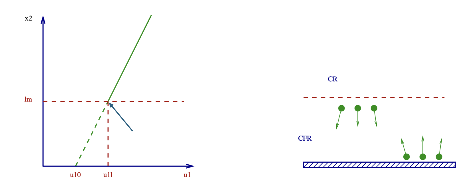
flux matching model:
we can use a flux matching model, can split the fluid regime into two regions

• Continuum zone: where molecules collide with each other frequently.

• Collision free zone, an area within one mean free path, where the particles more frequently collide with the wall than each other.

• In reality there is a gradual variation.

looking at momentum transfer to the wall

• Our momentum carried in the x₁ direction to the wall is:

  • \text{Flux of }x_1\text{-momentum from incident molecules}=\frac{\rho\bar{C} u_{1\lambda}}{4}

• Out momentum carried in the x₁ direction away from the wall:

  • Now this depends, on how our molecules reflect. If they bounce perfectly (specular) then no x₁ momentum is lost. But if they bounce off in a diffuse pattern, then momentum is lost. Thus:

  • \text{Flux }x_1\text{-momentum from reflected molecules}=\frac{(1 - \alpha_m) \rho\bar{C} u_{1\lambda}}{4}

  • There is an Momentum Accommodation Factor (\alpha_m):

Our change in momentum is thus:

\text{Net flux} = \frac{\alpha_m \rho \bar{C} u_{1\lambda}}{4}

looking at momentum transfer into the collision free zone

\text{ flux }x_1\text{-momentum carried through plane }(x_2=\lambda)=\mu\frac{du_1}{dx_2}=\frac{\rho\bar{C} \lambda}{2}\frac{du_1}{dx_2}

• This comes from the viscosity expression

derivation of slip

Now equating our two expressions, because of steady state our momentum within the collision free zone must stay the same. We get

2\lambda\frac{du_1}{dx_2}=\alpha_{m}u_{1\lambda}=\alpha_{m}\left(u_{10}+\lambda\frac{du_1}{dx_2}\right)

• We’re converting to u_{1\lambda} our velocity at the boundary between the two zones, into the wall velocity and an extrapolated term.

Working out our extrapolated surface velocity now:

u_{10}=\left(\frac{2 - \alpha_m}{\alpha_m}\right)\lambda\frac{du_1}{dx_2}

Now with some basic dimensional analysis, our local velocity gradient:
\frac{du_1}{dx_2} = \frac{u_{1\infty}}{L}

so can get the equation

\frac{u_{10}}{u_{1\infty}}=\left(\frac{2 - \alpha_m}{\alpha_m}\right)\frac{\lambda}{L}

• No slip condition valid as long as our length scales much larger than mean free path

• Also obviously invalid if our momentum accomodation coefficient is close to zerok

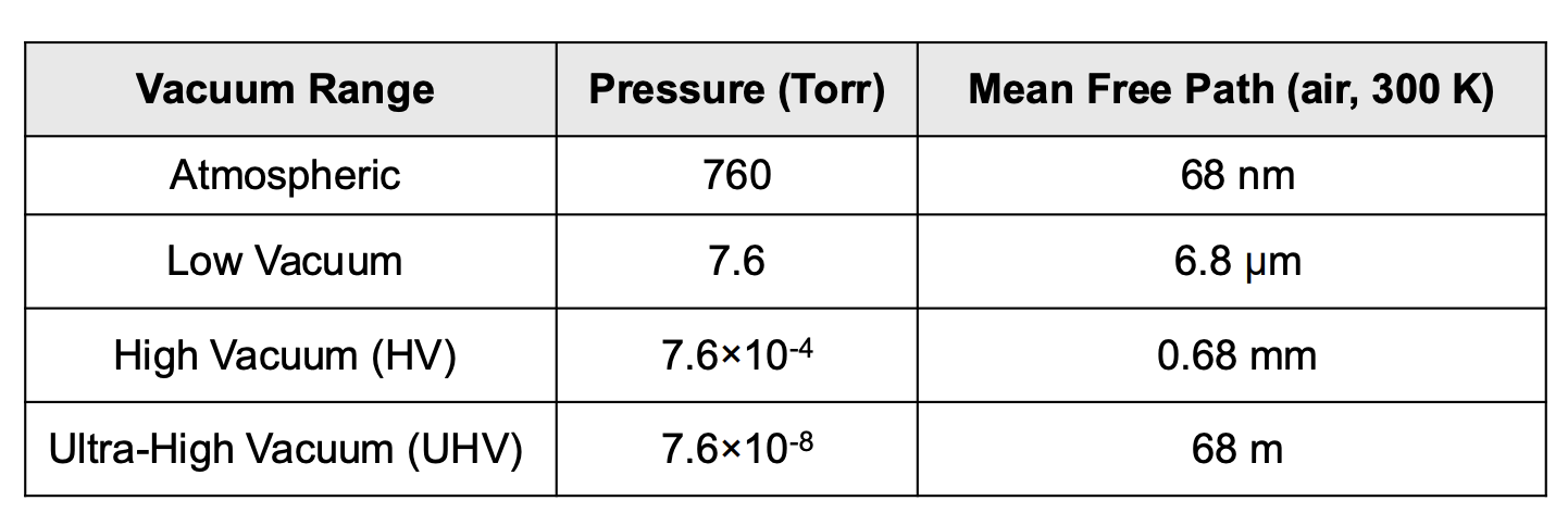
Knudsen number

The ratio of the mean free path to our system characteristic length is defined as the Knudsen number
Kn = \frac{\lambda}{L}

different flow regimes

Regime	Range of Kn	Physics Description	Mathematical Tool
Continuum	Kn < 0.01	Molecules collide so often they act as a single unit.	Navier-Stokes (No-Slip)
Slip	0.01 < Kn < 0.1	The gas acts as a fluid, but starts "slipping" at the walls.	Navier-Stokes + Slip BCs
Transition	0.1 < Kn < 10	Collisions and free flights are equally important. (difficult to analyse)	Boltzmann Equation
Free-Molecule	Kn > 10	Molecules hit walls but rarely hit each other.	Collisionless Kinetic Theory

note on boundary layer analysis

note that our boundary layer analysis only really makes sense in the slip and continuum regimes, as viscosity sort of becomes irrelevant with free molecular flows

Knusden number and couette flow

To illustrate how knusden number affects the flowfield we will look at couette flow (flow between a moving plate and stationary plate, with uniform pressure

continuum case

• Here we get a linear velocity profile with a constant shear stress given by:

• [\tau_0]_{cont} = \frac{\mu U}{L} = \frac{\rho \bar{C} \lambda U}{2 L}

  • We are replacing μ with the kinetic theory definition of \frac{1}{2}\rho \bar{C} \lambda

• if we remember correctly this is just either simplifying navier stokes or a control volume

free molecular analysis

This is now taking the extreme case where kn»1, the particles don’t hit each other, just the wall

• We will assume an accommodation coefficient of 1, with perfect diffuse reflection (so the mean velocity equals the wall velocity)

• No momentum transfer from bottom to top, as the mean x1 velocity is zero

• momentum transfer from top to bottom is: \frac{\rho \bar C U}{4} , this is the flux from particles moving at an average speed equal to the plate.

Thus momentum transfer per unit area is equal to shear stress and equal to:

[\tau_0]_{fm}=\frac{\rho\bar{C}U}{4}

difference between scenarios

we can see the difference in our shear stress if we combine the two equations is:

\frac{[\tau_0]_{fm}}{[\tau_0]_{cont}}=\frac{1}{2 Kn}{}

• In free molecular regime shear stress gets increasingly small.

• the approximate variation is shown in the graph

high knusden number scenarios

• Very low densities (rarefied gas dynamics)

• Very small scales like in MEMs or with aerosols and nano particles
  

Introduction to stat mech:

• Statistical mechanics is a “bigger” picture and only tells us about equilibrium states and not about rates

• We can derive our classical equations of state from statistical mechnics

• Give a physical basis for the first and second laws of thermodynamics.

Statistical behaviour of large systems

Real systems involves vast numbers of states on the order of the avagadro’s number, discrete states are given by quantum mechanics.

Microstates vs macrostates:

A microstate is all the information needed to describe a system, using large numbers of quantum numbers to describe energy levels, translation, rotation, vibration etc.

• This is an unreasonable amount of information

We are however generally interested in a broader picture of systems, like the pressure, temperature. These broader average quantities are subject to fluctuations but they are small.

These are our macro states

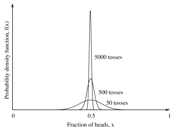
coin tossing analogy

Imagine tossing a coin 4 times in a row,

• each sequence like HTHT can be considered our microstate.

• Our macrostate is the number of heats for example.

Macrostate (Total Heads)	Microstates (Specific Sequences)	Number of Microstates (W)
0 Heads	TTTT	1
1 Head	HTTT, THTT, TTHT, TTTH	4
2 Heads	HHTT, HTHT, HTTH, THHT, THTH, TTHH	6
3 Heads	HHHT, HHTH, HTHH, THHH	4
4 Heads	HHHH	1
Total	—	16

• As we increase the number of tosses, such as for a large system, the distribution becomes sharper.

• System is becomes increasingly defined by its most probable macrostate

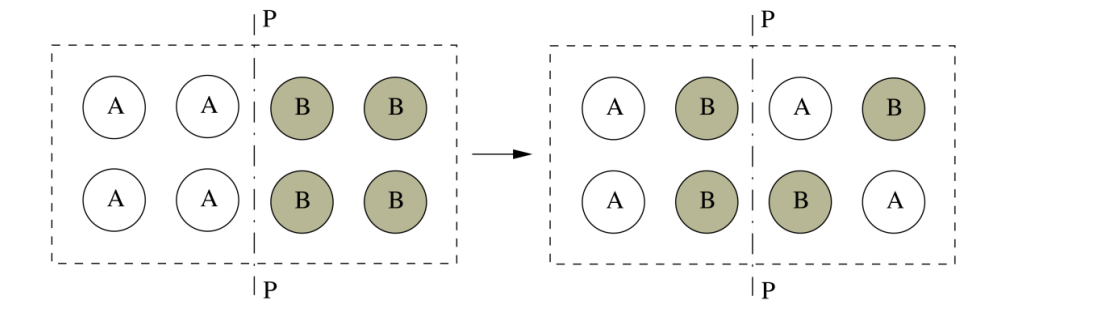
Macro state example, crystal mixing analogy.

We can see an example of how macro states can vary with this simplified model of a crystal.

• The macrostate is given by the of atoms left of plane P-P

We can use the CHOOSE function \binom{n}{k} = \frac{n!}{k!(n-k)!}. to define how many ways of arranging our B atoms are in each state, allowing us to calculate the number of microstates in each macrostate.

Macrostate	B atoms on Left	Ways to pick B's on Left	Ways to pick B's on Right	Total Microstates (W)
1	0	\binom{4}{0} = 1	\binom{4}{4} = 1	1 \times 1 = \mathbf{1}
2	1	\binom{4}{1} = 4	\binom{4}{3} = 4	4 \times 4 = \mathbf{16}
3	2	\binom{4}{2} = 6	\binom{4}{2} = 6	6 \times 6 = \mathbf{36}
4	3	\binom{4}{3} = 4	\binom{4}{1} = 4	4 \times 4 = \mathbf{16}
5	4	\binom{4}{4} = 1	\binom{4}{0} = 1	1 \times 1 = \mathbf{1}
TOTAL				70

notes:

• We can see the mixed macrostate 3 is the most probable. As the number of atoms increase, at equilibrium the mixed macrostate is the only one we will ever see

• This is because the distribution becomes sharper with more atoms

• this model can be used to calculate the entropy of mixing

Fundamental statistical posulate