Anticipating Patterns

probability

a measure of the likelihood of an event

sample space

a set of all possible outcomes of an experiment (ex. for rolling a 6-sided die: S = {1, 2, 3, 4, 5, 6}

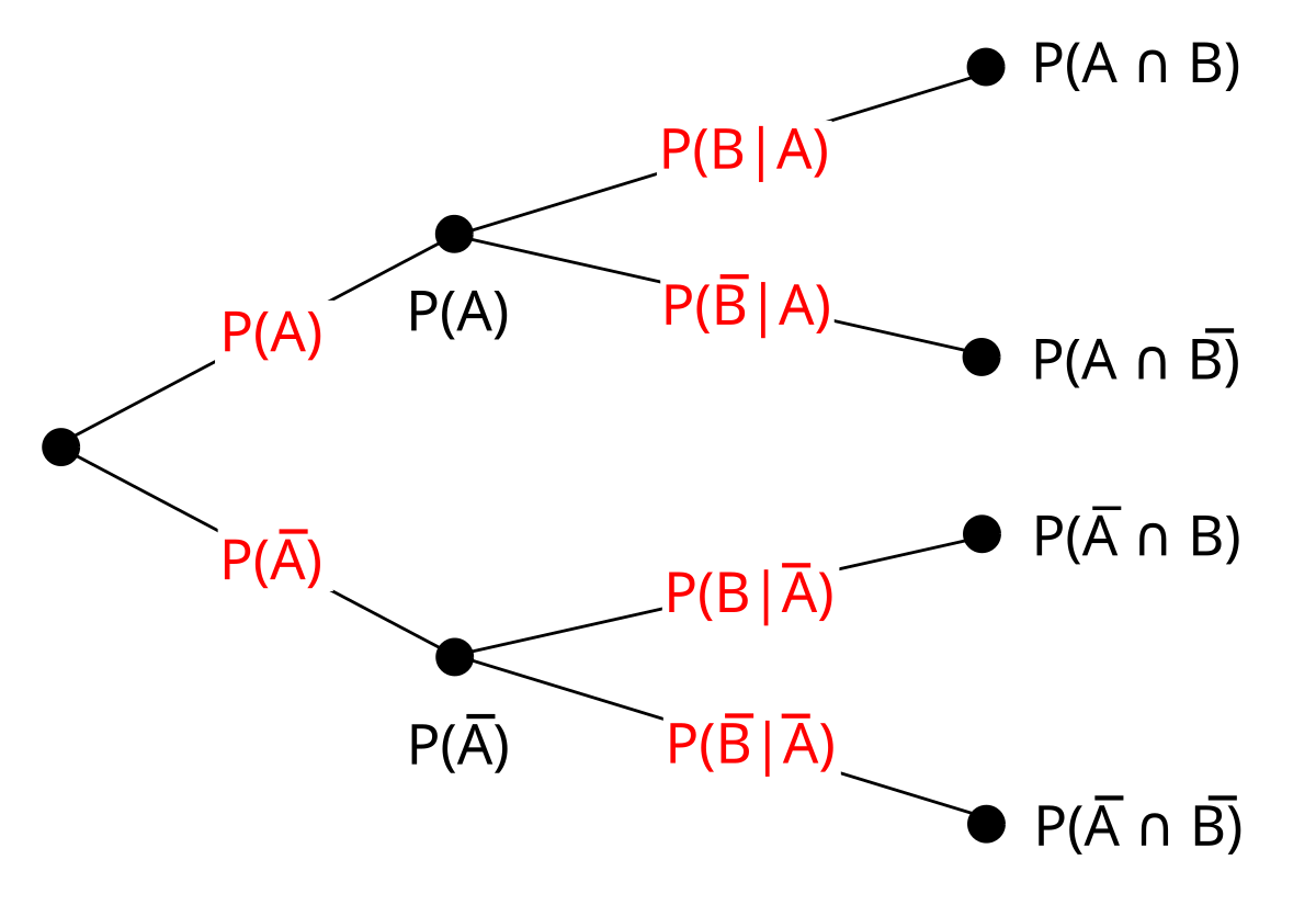
tree diagram

a representation used to determine the sample space for an experiment

event

an outcome or set of outcomes of a random phenomenon - a subset of the sample space

impossible event

an event that can never occur, with a probability of 0

sure event

an event that must occur every time, with a probability of 1

odds in favor of an event

a ratio of the probability of the occurrence of an event to the probability of the nonoccurrence of that event: P(Event A occurs)/P(Event A does not occur) or P(occurs) : P(doesn’t occur)

complement

the set of all possible outcomes in a sample space that do not lead to the event. for event A, denoted by A’

disjoint/mutually exclusive events

events that have no outcome in common, and cannot occur together

union

the set of all possible outcomes that lead to at least one of the two events A and B. for events A and B, denoted by (A∪B) or (A or B)

intersection

the set of all possible outcomes that lead to both events A and B. for events A and B, denoted by (A∩B) or (A and B)

conditional event

A given B is a set of outcomes for event A that occurs only if B has occurred. for events A and B, denoted by (A|B)

independent events

when the occurrence of one event does not affect the probability of the other event. for events A and B, P(A) should equal P(A|B)

variable

a quantity whose value varies from subject to subject (e.g. height, number of home runs hit in a season, hair colors, altitude of an airplane in flight, etc.)

probability experiment

an experiment whose possible outcomes may be known but whose exact outcome is a random event and cannot be predicted with certainty in advance

random variable

a numerical outcome of a probability experiment

discrete random variable

a quantitative variable that takes a countable number of values (e.g. no. of emails received per day, no. of home runs per batter, no. of red blood cells per sample of blood, etc.) - there cannot be part of a unit of the variable (no possibility of 0.67 of an email sent)

continuous random variable

a quantitative variable that can take all the possible values in a given range (e.g. weight, plane altitude, amount of rainfall, etc.)

probability distribution of a discrete random variable/discrete probability distribution

a table, list, graph, or formula giving all possible values taken by a random variable and their corresponding probabilities

expected value

the mean of a discrete random variable, denoted by E(X) and computed by multiplying each value of the random variable by its probability and then adding over the sample space

variance of a discrete random variable

the sum of the product of squared deviations of the values of the variable from the mean and the corresponding probabilities

combination

the number of ways r items can be selected out of n items if the order of selection is not important. denoted by (n choose r) and computed as (n!) / [r! (n-r)! ]

binomial probability distribution

number of trials is fixed, number of successes is random. calculates the probability of x successes in n trials. computed with P_x = (n x)p^x(q)^n-x

geometric probability distribution

number of successes is fixed, number of trials is random. occurs in an experiment where there are n repeated trials, each trial is a bernoulli trial, trials are repeated until a predetermined number of successes is reached, and all are identical and independent. computed with P(x trials needed until first success) = (1-p)^x-1p

mean of geometric random variable

μ = E(X) = 1/p

variance of geometric random variable

σ² = Var(X) = (1-p)/p²

probability distribution of a continuous random variable/continuous probability distribution

a graph or formula giving all possible values taken by a random variable and the corresponding probabilities. also known as the density function or probability density function (pdf)

cumulative distribution function (cdf)

calculates for a random variable X P(X ≤ x₀).

mean and variance for combined variables

for X-Y, μ = μ_x - μ_y and σ² = σ²_x + σ²_y. for X+Y, variance is the same, but μ = μ_x + μ_y. if X and Y are normally distributed, then a linear combination of the two will also be normally distributed

normal distribution/bell curve/Gaussian distribution

the most commonly used distribution in statistics, closely approximates the distributions of many different measurements with a continuous, unimodal, and symmetric curve. if random variable X follows a normal distribution with mean μ and standard deviation σ, it is denoted by X ~ N(μ, σ). (~ is “is distributed as”)

standard normal

the normal distribution with a mean of 0 and a standard deviation of 1. any normal random variable can be transformed into the standard using Z = (X - μ)/σ, meaning Z ~ N(0, 1) → X = Zσ + μ ~ N(μ, σ)

z-score

the value of variable Z computed as Z = (X - μ)/σ for any specific value of X. (e.g. if X~N(10,2), the z-score for X = 12.5 is (12.5-10)/2 = 1.25)

probability for a one-tailed z-score of 95%

1.645

probability for a two-tailed z-score of 95%

1.96

probability for a one-tailed z-score of 99%

2.33

probability for a two-tailed z-score of 99%

2.58

when to use invNorm

when you have an area under the curve to the left of a value and need to know the value

when to use normalcdf

when you have a range of values to find the area under the curve for

central limit theorem

regardless of the shape of the distribution of the population, if the sample size is large (usually greater than or equal to 30) and there is finite variance, then the distribution of the sample means will be approximately normal, with mean μ_x = μ and standard deviation σ_x = σ/√n.

as the sample size n increases, the distribution of X becomes more symmetric, with the center remaining at μ and the spread decreasing with the distribution peaking

sampling distribution of a sample proportion

with a large n, the sampling distribution of p̂ is approximately normal, with mean μ_p̂ = p and standard deviation σ_p̂ = √[p(1-p)]/n

sampling distribution of a sample mean

for a large n, the sampling distribution of X̄ is approximately normal, with mean μ_X̄ = μ and standard deviation σ_X̄ = σ/√n

sampling distribution of a difference between two independent sample proportions

for large sample sizes, the sampling distribution of (p̂₁ - p̂₂) is approximately normal, with mean μ_{p̂1 - p̂2} = p₁ - p₂ and standard deviation σ_{p̂1 - p̂2} = √ [p₁(1-p₁)]/n₁ + [p₂(1-p₂)]/n₂

sampling distribution of a difference between two independent sample means

for a large n₁ and n₂, the sampling distribution of (X̄₁ - X̄₂) is approximately normal, with mean μ_{X̄1 - X̄2} = μ₁ - μ₂ and standard deviation σ_{X̄1 - X̄2} = √ [σ₁² / n₁] + [σ₂² / n₂]

confidence intervals/confidence levels

consists of two numbers between which you can be reasonably certain the true parameter will fall

statistical hypothesis

a claim or statement about a parameter value. always a statement about a population characteristic and not about a sample

null hypothesis

a statement that is assumed to be true until proven otherwise

alternative hypothesis

a statement about the parameter that must be true if the null hypothesis is false

test statistic

a statistic computed from the sampled data and used in the process of testing a hypothesis. (e.g. if using a normal model, the test statistic is the z-score)

p-value

the probability that a test statistic value would be observed by chance, given the null hypothesis is true

alpha level

a predetermined cutoff point for what is to be considered a statistically significant p-value. commonly 0.05

type i error

the error of rejecting the null hypothesis when it is true (false positive)

type ii error

the error of failing to reject the null hypothesis when it is false (false negative)

power of a test

the probability of correctly detecting an effect when there really is an effect. increases as the sample size increases, as the type i error rate (α) increases, and as the effect size increases

effect size

the difference between the hypothesized value of a parameter and its true value

rejection region/critical region

the set of test statistic values for which the null hypothesis should be rejected. the area of this region is equal to α

non-rejection region

the set of test statistic values for which there should be a failure to reject the null hypothesis

critical value

the value of a test statistic that gives the boundary between the rejection and non-rejection region. denoted as z* or t*

left-tailed test

used when 'too-small’ values of the statistic as compared to the hypothesized parameter value lead to the rejection of the null hypothesis. the entire rejection region falls in the left tail of the sampling distribution of the test statistic

right-tailed test

used when ‘too-large’ values of the statistic as compared to the hypothesized parameter value lead to the rejection of the null hypothesis. the entire rejection region falls in the right tail of the sampling distribution of the test statistic

two-tailed test

used when both ‘too-small’ and ‘too-large’ values of the statistic as compared to the hypothesized parameter lead to the rejection of the null hypothesis. the rejection region falls in both tails of the sampling distribution of the test statistic, generally being divided equally

computing sample size

when computing sample size, always round up. often will need to find the value for the z-score, where the critical z-score is denoted as z*, and computed with the tail area equaling α

determining the sample size to estimate population mean μ

ME = z*(σ/√n)

determining the sample size to estimate population proportion

ME = z*√[p(1-p)]/nk

how are sample sizes affected by different changes

sample size increases with a decrease of margin of error, increase of confidence level, and increase of standard deviation

estimation procedures

used to estimate unknown population parameters, such as constructing confidence intervals

inference procedures

used for testing claims about unknown population parameters, such as testing hypotheses

when to use t-distribution

when the population standard deviation is unknown and the sample size is small

when to use normal distribution

when the population standard deviation is known

t-distribution

a continuous, symmetric distribution, with a mean of 0 and a bell-shaped curve. its shape depends on degrees of freedom - for a smaller df, the distribution is more spread with thicker tails. as the df gets larger, the tails get thinner and the distribution looks more like the normal distribution. as the df increases, the standard deviation increases

sampling distribution of x̄

if the population is normally distributed and the population standard deviation is known, then the sampling distribution of x̄ is also a normal distribution. if the population is normally distributed and the population standard deviation is unknown, then the sampling distribution of x̄ is a t-distribution with (n-1) degrees of freedom

observed frequency

the number of measurements from one experiment falling into that particular cell

expected frequency

the number of measurements expected to fall into the cell according to our theory

least-squares regression technique

where the slope and Y-intercept can be estimated from n pairs of measurements as b = r s_y/s_x and a = ȳ - bx̄. a becomes alpha and b becomes beta

error/residual

the difference between the observed response and the response predicted by the estimated regression line