Chapter 18- Biogeography

Biogeography

the study of patterns of species composition and diversity across geographic locations.

Patterns of species diversity and distribution vary at…

global, regional, landscape, and local spatial scales

Spatial scales are interconnected in a …

hierarchical way

The patterns of species diversity and composition at one spatial scale set…

the conditions for patterns at smaller spatial scales.

What 3 factors influence global patterns of species diversity

1. Geographic area and isolation

2. evolutionary history

3. global climate.

Endemic

Spp do not occur anywhere else on earth

Rank species richness -of forest location and types

1. Amazon, Brazil (1,300

2. Southern California, US (57)

3. Beech Forest, NZ (20)

4. Pacific Northwest, US (7,4)

5. Boreal Forest, Canada (2)

What can we conclude about biogeographic patterns on Earth, assuming that forest communities are good global representatives?

1. Species richness and composition vary with latitude: the lower tropical latitudes have many more, and different, species than the higher temperate and polar latitudes.

2. Species richness and composition vary from continent to continent, even where longitudes or latitudes are roughly similar.

3. The same community type or biome can vary in species richness and composition depending on its location on Earth.

Figure 18.5- Interconnected Spatial Scales of Species Diversity

Rank Spatial Scales from highest to lowest

1. Global Scale

2. Regional Scale

3. Landscape Scale

4. Local Scale

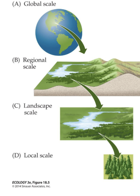
Global Scale includes

the entire world

Components of Global Scale

• Species have been isolated from one another, on different continents or in different oceans, by long distances and over long periods.

• Rates of speciation, extinction, and dispersal help determine differences in species diversity and composition

Regional scale

• areas with uniform climate

• the species are tied to that region by dispersal limitations.

Regional species pool (gamma diversity)

all the species contained within a region

Landscape Scale

• topographic and environmental features of a region.

Components of Landscape Scale

• Species composition and diversity vary within a region depending on how the landscape shapes rates of migration and extinction.

Local scale (alpha diversity)

equivalent to a community.

Components of Local scale

• Species physiology and interactions with other
  species are important factors in the resulting
  species diversity.

Actual area of different spatial scales depends on…

the species and communities of interest

Example of how different spatial scales depends on the species and communities of interest

Terrestrial plants might have a local scale of 102–104 m2, but for bacteria, the local scale might be more like 102 cm2.

What is the species pool?

The set of all species contained within a region that can potentially colonize local sites.

3 types of species diversity

1. Gamma

2. Alpha

3. Beta

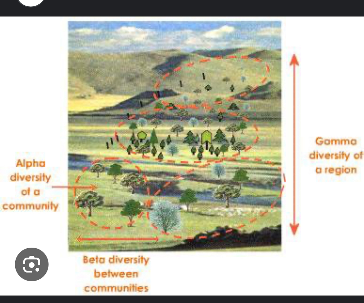
Gamma Species Diversity

Species diversity within a region

Alpha Species diversity

local species diversity of a community

Beta diversity

• Change in species number and composition, or turnover of species, from one community type to another (diversity btwn communities)

• connects local and regional scales.

• one moves from one community type to another across the landscape

The regional species pool provides

raw material for local assemblages and sets the theoretical upper limit on species diversity for communities.

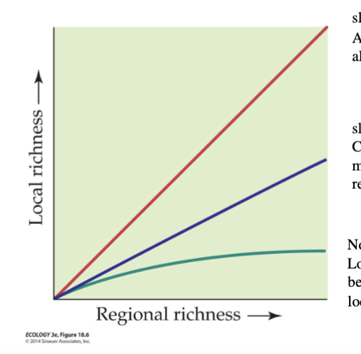
Figure 18.6- What determines local species richness

What does slope= 1 represent?

• Red

• When local and region spp richness values are equal, then all species in a region will be found in all communities

• Not feasible for real world because regions have varying landscape and habitat features

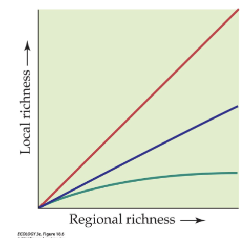
Figure 18.6- What determines local species richness

What does slope <1 represent?

• Blue

• When local richness values are lower than regional richness values by still increase with them proportionally, community richness is mostly determined by the regional species pool

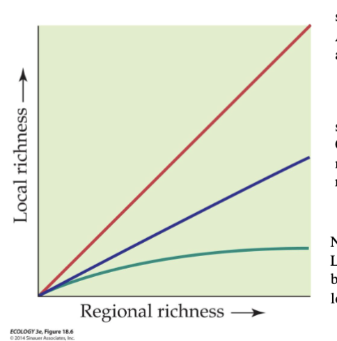
Figure 18.6- What determines local species richness

What does non-linear slope represent?

• Green

• I local richness stays the same as regional richness, local processes limit local species richness

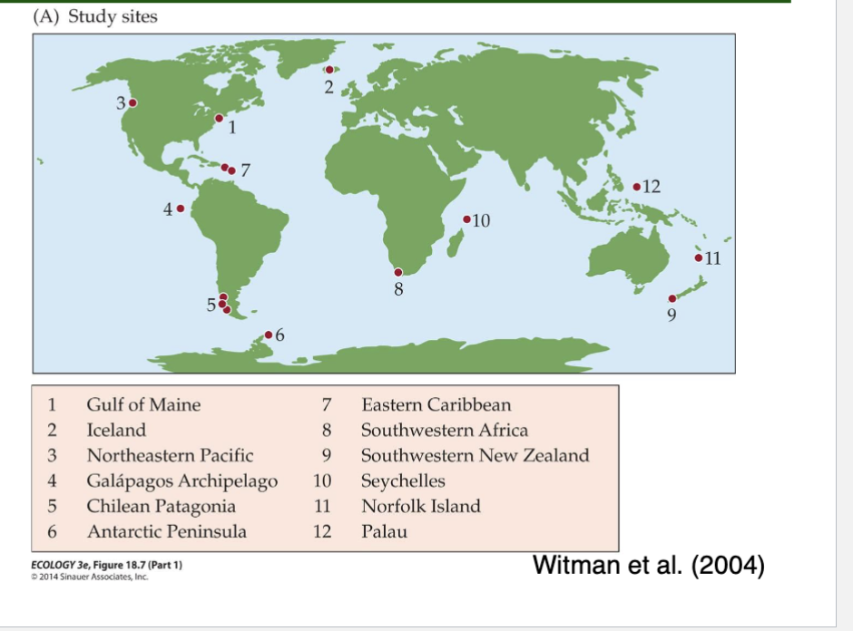
Figure 18.7 (A) - Wittman. Marine Invertebrate Communities May be Limited by Regional Processes Components

• Witman and colleagues (2004) considered this relationship for marine invertebrate communities living on subtidal rock walls at a variety of locations throughout the world

• At 49 local sites in 12 regions, they surveyed species richness of marine invertebrates on subtidal rock walls

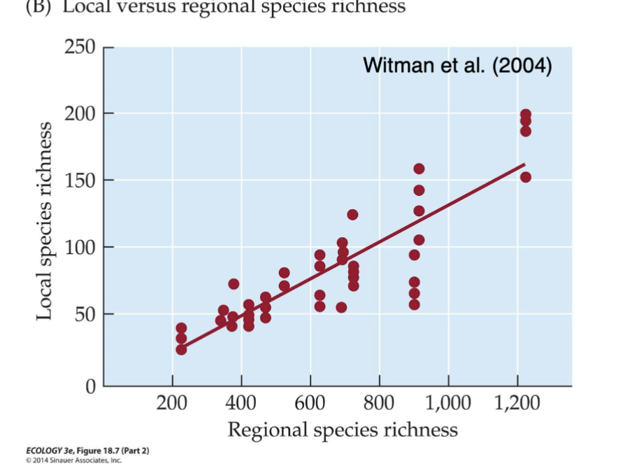
FIGURE 18.7B: Witman Marine Invertebrate Communities May be Limited by Regional Processes Components

Local vs Regional Species Richness Graph Components

• Important result:

  • Local species richness did not level off, even as regional species richness increased—meaning local communities did not reach saturation.

  • A statistical analysis showed that regional species richness explained approximately 75% of the variation in local species richness.

• This means that regional species pools (gamma diversity) largely determine the number of species present at the local scale (alpha diversity).

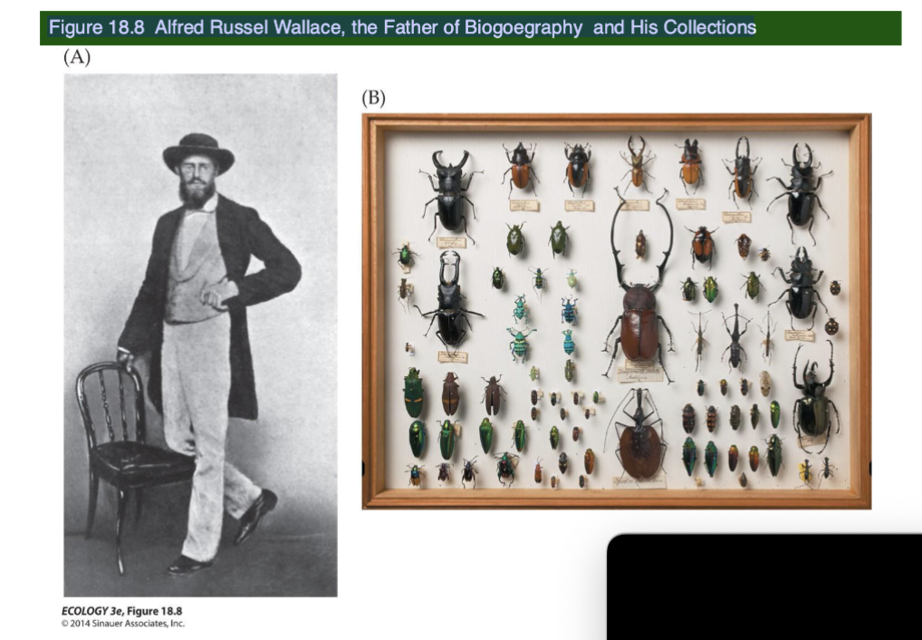
Figure 18.8 Alfred Russel Wallace, the Father of Biogoegraphy and His Collections

What did Wallace Find?

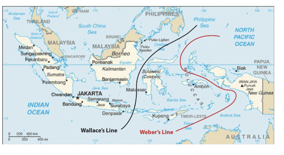
1. Wallace’s Line:

   • Wallace noticed a sharp boundary between the faunas of Asia and Australia in the Malay Archipelago (near Indonesia).

   • The Malay Archipelago: that the mammals of the Philippines were more similar to those in Africa (5,500 km away) than they were to those in New Guinea (750 km away).

2. Wallace’s Two Major Global Patterns:

   • Earth’s land masses can be divided into six recognizable biogeographic regions containing distinct biotas that differ markedly in species diversity and composition.

   • There is a gradient of species diversity with latitude: species diversity is greatest in the tropics and decreases toward the poles.

Biographic Regions

Regions that contain distinct biotas that differ markedly in species diversity and composition

What does this image depict?

• Wallace’s Line (black line):

  • Drawn by Alfred Russel Wallace in the 1800s.

  • It marks a sharp boundary between the fauna of Asia (left/west) and the fauna of Australia (right/east).

  • Example:

    • To the west (like Borneo, Sumatra, and Java): mammals like tigers, elephants, and monkeys (Asian fauna).

    • To the east (like New Guinea and Australia): marsupials like kangaroos and tree kangaroos (Australian fauna).

• Weber’s Line (red line):

  • Drawn later by Max Weber.

  • It is a more refined, gradual boundary that runs farther east.

  • It shows that species mixing is more complex, not as sharp as Wallace originally thought, with some overlap (species transition zone).

• Geographic Area Covered:

  • Southeast Asia and Oceania, including islands like Borneo, Sulawesi, New Guinea, and the Philippines.

Why This is Important:

• Historical reason: The sharp difference in animal species occurs because of deep water channels that never dried up, even during ice ages when sea levels were lower.

• Evolutionary reason: Species evolved separately for tens of millions of years on the Asian and Australian continental plates.

• Biogeographic reason: It proves that physical barriers like oceans can create huge biodiversity differences even across short distances.

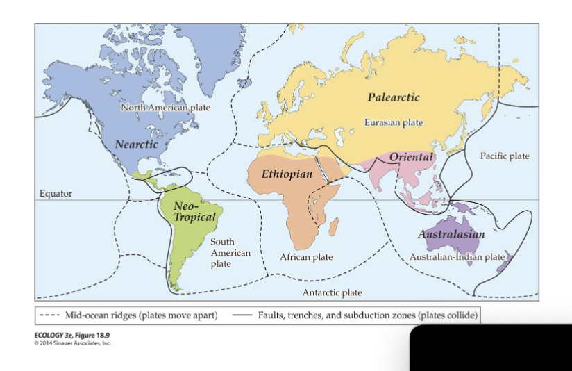
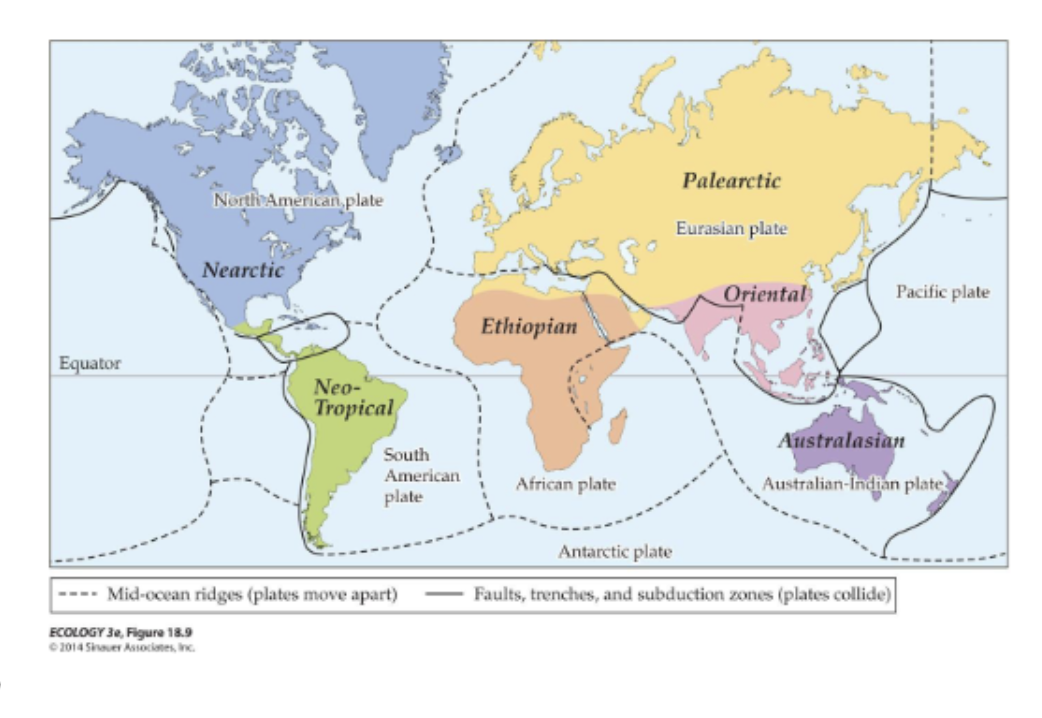
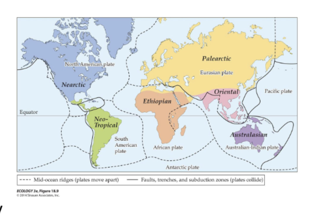
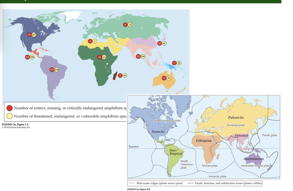
Figure 18.9- Six Biographical regions

What did Wallace’s Book: The Geographical Distribution of Animals (1876) identify using the distributions of terrestrial animals

• The land masses can be divided into 6 biogeographic regions which conicide with earth’s major 6 tectonic plates

• There is a gradient of species diversity with latitude

Tectonic Plates

• sections of Earth’s crust that move across Earth’s surface through the action of currents generated deep within its molten rock mantle

Continental drift

• The process that drive the movement of tectonic plates

• Hypothesized that the continents drifted over Earth’s surface

Three major types of boundaries between tectonic plates.

1. Mid-ocean ridges

2. Seafloor Spreading

3. Subduction Zone

Mid-Ocean Ridges

• molten rock flows out of the seams between plates and cools, creating new crust and forcing the plates apart

Seafloor Spreading

New crust and forcing the plates apart in a process called

Subduction Zone

• Area where 2 plates meet

• One plate is forced downward under another plate.

• These areas are associated with strong earthquakes, volcanic activity, and mountain range formation

Fault

• Areas where two plates meet, the plates slide sideways past each other

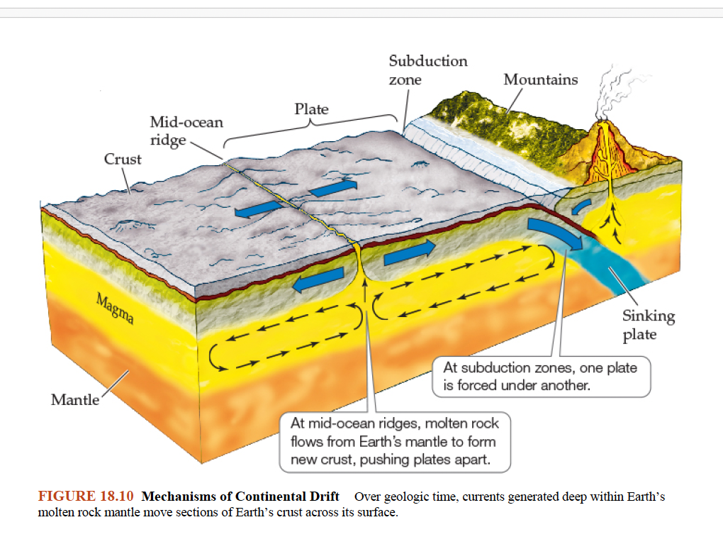
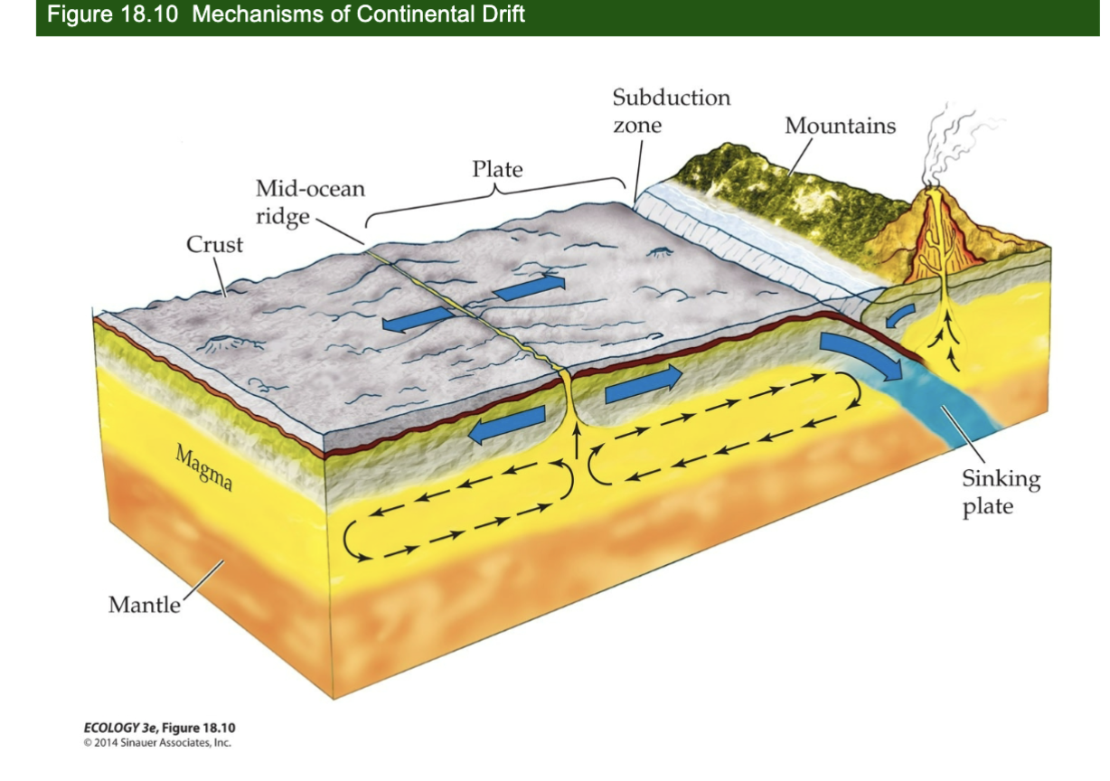
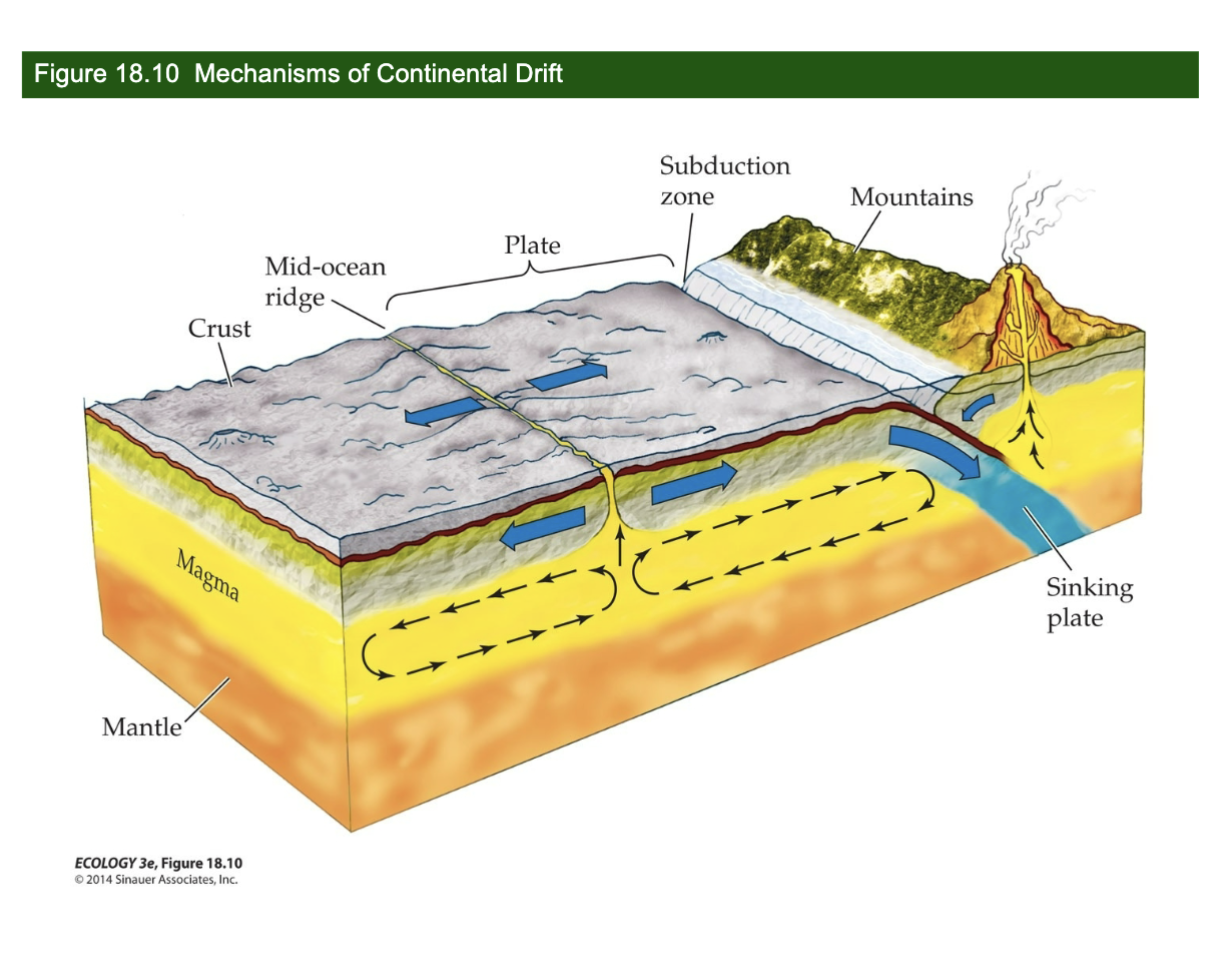
Figure 18.10- Mechanisms of Continental Drift

• As a result of processes such as seafloor spreading and subduction, the positions of the plates, and of the continents that sit on them, have changed dramatically over geologic time

How does continental drift work, and why is it important in biogeography?

Convection currents in Earth's mantle move tectonic plates, forming mid-ocean ridges and subduction zones. Continental drift separated species over millions of years, driving evolutionary divergence and creating distinct biogeographic regions.

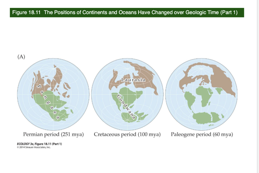
Explain Figure 18.11- The Positions of Continents and Oceans Have Changed over Geologic Time

Permian Period (251 million years ago)

• Supercontinent Pangaea existed.

• All the continents were fused together into one giant landmass.

• Species could move freely across connected land areas.

• Very little geographic isolation at this point.

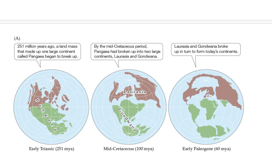
Explain Figure 18.11- The Positions of Continents and Oceans Have Changed over Geologic Time

Early Triassic Period (251 mya)

• When all of Earth’s land masses, a single continent named Pangaea, began to break up

• At that time, there was a mass extinction which eventually led to the rise of the first archosaurs (precursors to dinosaurs) and the cynodonts (precursors to mammals).

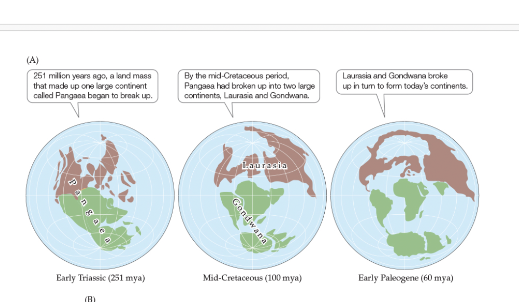
Figure 18.11- The Positions of Continents and Oceans Have Changed over Geologic Time

Mid- Cretaceous Period (100 mya)

• Pangaea split into two massive continents:

  • Laurasia in the north (North America, Europe, Asia)

  • Gondwana in the south (South America, Africa, Antarctica, Australia, India)

• Significant isolation began between northern and southern species.

• Ocean basins started widening.

• Divergence of species accelerated because of geographic separation.

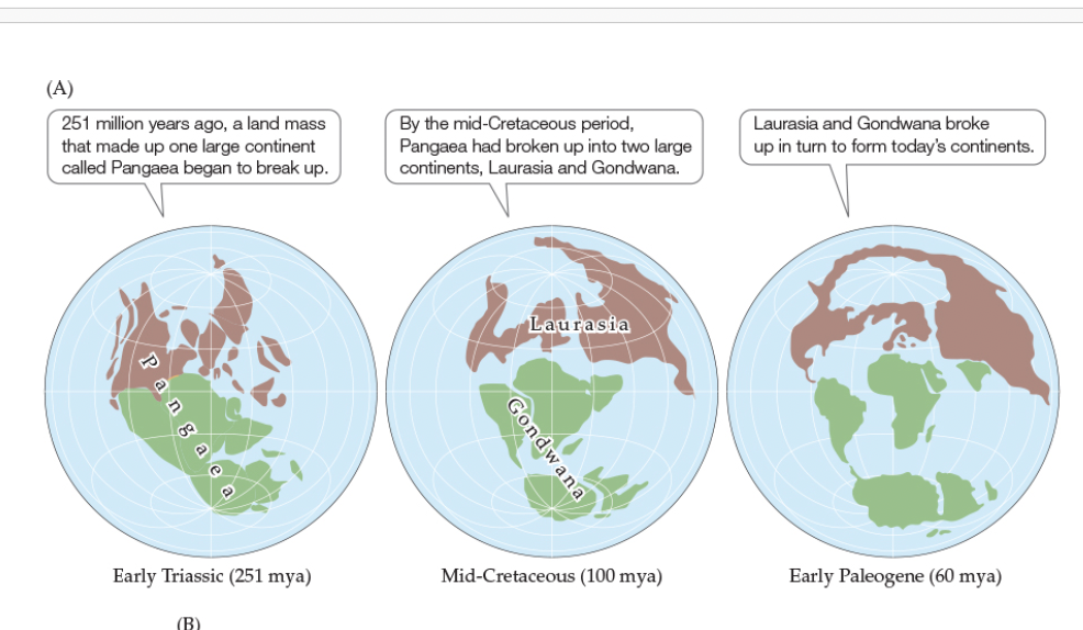
Figure 18.11- The Positions of Continents and Oceans Have Changed over Geologic Time

Early Paleogene Period (60 mya)

• Gondwana had separated into the present-day continents of South America, Africa, India, Antarctica, and Australia. Laurasia eventually split apart to form North America, Europe, and Asia. Most of these movements resulted in the separation of continents from one another, but some continents were brought together

• For example, North and South America joined at the Isthmus of Panama, India collided with Asia to create the Himalayas, Africa and Europe united at the Mediterranean Sea, and a land bridge formed between North America and Asia at the Bering Strait

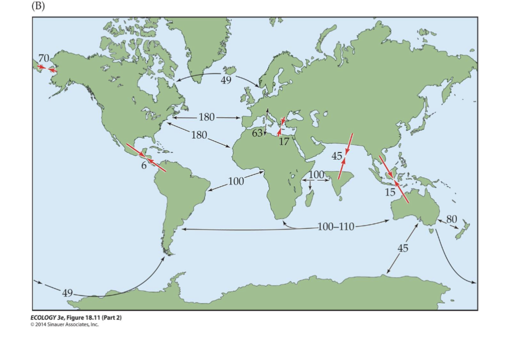
Explain Figure 18.11 (B) The Positions of Continents and Oceans Have Changed over Geologic Time

• A summary of the movements that led to the configuration of the continents we know today. Red arrows are labeled with the time (in millions of years) since land masses joined; black arrows are labeled with the time since land masses separated.

• Key Takeaways:

  • Continental drift continues today — it wasn't just ancient history!

  • The positions of continents have changed dramatically even in the last 100 million years.

  • These movements:

    • Created new barriers (oceans).

    • Allowed species mixing in some cases (like India colliding into Asia).

    • Drove evolutionary changes by separating or joining different biotas.

The Neotropical, Ethiopian, and Australian regions…

have been isolated for a long time and have very distinctive forms of life

The Nearctic region differs substantially from the Neotropical despite…

modern- day proximity.

North America was part of…

Laurasia

South America was part of …

• Gondwana.

• They had no contact until about 6 million years ago; there has been some movement of
  species since then.

The main question, then, is whether there are barriers to dispersal between oceans as there are between continents.

• Despite their appearance of connectivity, oceans do have significant impediments to the exchange of biotas: these impediments take the form of continents and currents; thermal, salinity, and oxygen gradients; and differences in water depth.

• Oceanographic discontinuities have isolated species from one another, allowed for evolutionary change, and created unique oceanic biogeographic regions

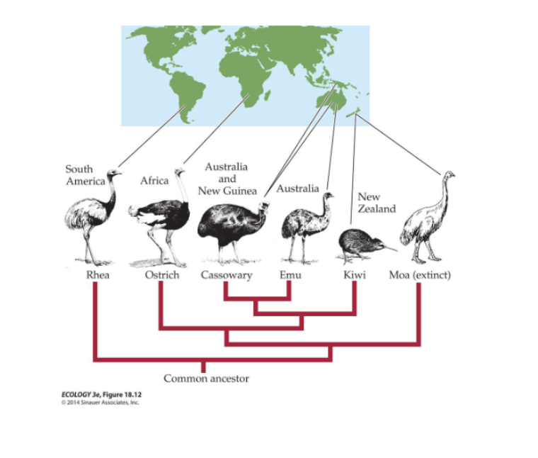
Vicariance

evolutionary separation of species by barriers such as those formed by continental drift

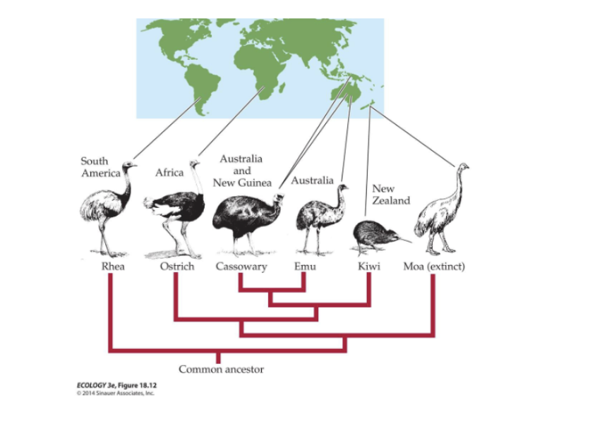
Explain this image

It shows the evolutionary relationships and geographic distribution of a group of large, flightless birds known as ratites

What is the difference between the Holt et al. (2013) biogeographic regions and the classic six-region model?

• Holt used phylogenetic information acquired from DNA analysis and recent observations of global species distribution patterns to test whether Wallace’s original biogeographic regions are supported by modern data. The researchers identified more biogeographic regions (a total of 11), some of which were the same and others of which were different from Wallace’s original 6 regions.

• This new analysis suggest sthat additional isolation mechanisms beyond continental drift are responsible for the different regions.

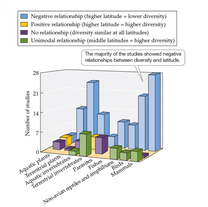
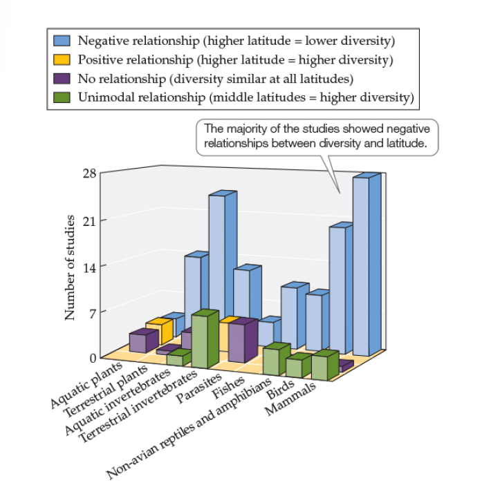
FIGURE 18.12 Willig Studies of Latitude and Species Diversity Confirm Conventional Wisdom

• Tallied the results of 162 studies on a variety of taxonomic groups extending over broad spatial scales (20° latitude or more) that considered whether diversity and latitude showed a

  1. negative relationship (with diversity decreasing toward the poles)

  2. positive relationship (increasing toward the poles)

  3. unimodal relationship (increasing toward mid-latitudes and then declining toward the poles)

  4. no relationship.

Results of Willig and Collegues Experiment

• Negative relationships were by far the most common.

• Strong Negative Relationship:

  • For almost every group, the majority of studies (blue bars) showed a negative relationship between latitude and species richness.

  • This confirms the classic latitudinal diversity gradient: more species near the equator, fewer toward the poles.

• Few Positive Relationships:

  • Very few studies (orange bars) found higher diversity at higher latitudes.

• Some Unimodal Patterns:

  • Some groups (especially fishes and invertebrates) showed a unimodal pattern — diversity was highest at mid-latitudes rather than exactly at the equator.

• Very Few “No Relationship” Results:

  • Very few studies found no trend (purple bars are small).

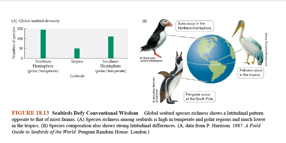
Explain Figure 18.13- Seabirds Defy Conventional Wisdom Global:

Guide to Seabirds of the World. Penguin Random House: London

• Seabirds have their highest diversity at temperate and polar latitudes

  • Seabirds of the Antarctic and subantarctic include penguins, albatrosses, petrels, and skuas. In the Arctic and subarctic, auks replace penguins, and gulls, terns, and grebes are common.

• In the tropics and subtropics, seabird diversity declines:

  • the seabird community is composed of pelicans, boobies, cormorants, and frigate birds.

• This pattern of seabird diversity correlates well with marine productivity, which is substantially higher in temperate and polar oceans than in the tropics

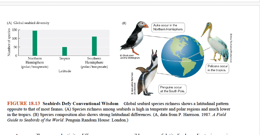
Why do seabirds show highest species richness at temperate and polar latitudes, contrary to most faunas?

• Because marine productivity is highest at temperate and polar regions, providing more food for seabirds.

• Most life = richest near the equator
  🐧 Seabirds = richest near the poles because that’s where the fish are!

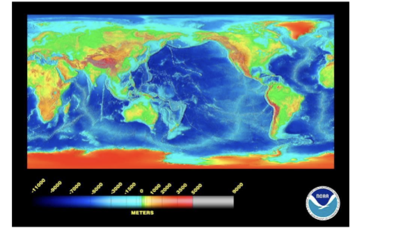
Identification of marine regions has been hindered by which 2 things?

1. the complicating factor of water depth

2. basic lack of knowledge of the deep oceans.

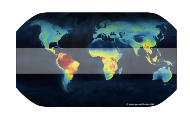
Biodiversity Hotspots

• Regions with exceptionally high biodiversity that are under threat.

• They are characterized by a large number of endemic specie

Global patterns of species richness are controlled by rates of which 3 things?

1. speciation

2. extinction

3. dispersal

Change in species richness Formula

∆S = D - E

Components of Species Richness Formula

• ∆S is the change in species richness

• D is the diversification rate (number of new species produced)

• E is extinction rate (loss of existing species)

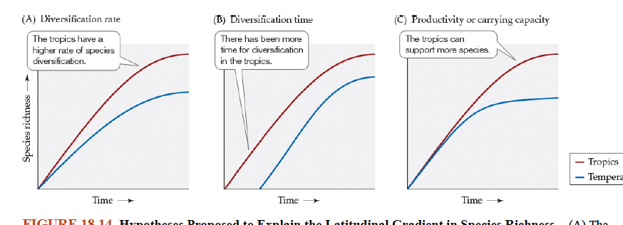
What are the three broad categories of hypotheses proposed by Mittelbach et al. (2007) to explain the latitudinal gradient in species richness?

1. Diversification Rate Hypothesis

2. Diversification Time Hypothesis

3. Productivity or Carrying Capacity Hypothesis

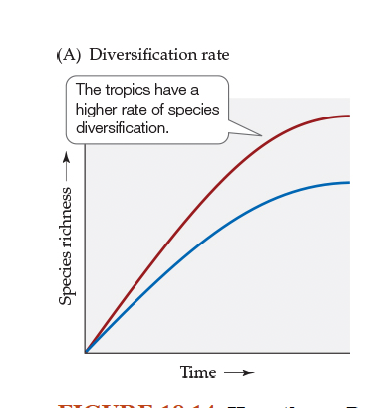
FIGURE 18.14 Gary Mittelbach Experiment Hypotheses Proposed to Explain the Latitudinal Gradient in Species Richness

Explain Figure A

• First category of hypotheses is based on the assumption that the

  • rate of species diversification in the tropics is greater than that in temperate regions

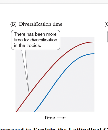
FIGURE 18.14 Hypotheses Proposed to Explain the Latitudinal Gradient in Species Richness

Explain Figure B

• The second category of hypotheses suggests that the

  • rates of diversification in the tropics and at higher latitudes are similar, but that the evolutionary time available for diversification has been much greater in the tropics

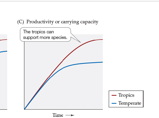
FIGURE 18.14 Hypotheses Proposed to Explain the Latitudinal Gradient in Species Richness

Explain Figure C

• The third category of hypotheses suggests that

  • resources are more plentiful in the tropics because of higher productivity, and thus that species there have higher carrying capacities and a greater ability to coexist

1. Species diversification rate

• The tropics have the most land area on Earth and temperatures are very stable.

• Large, thermally stable areas should decrease extinction rates—population sizes and geographic ranges would be larger.

• Speciation by geographic isolation would be more likely.

• Terborogh and Rosenzweig

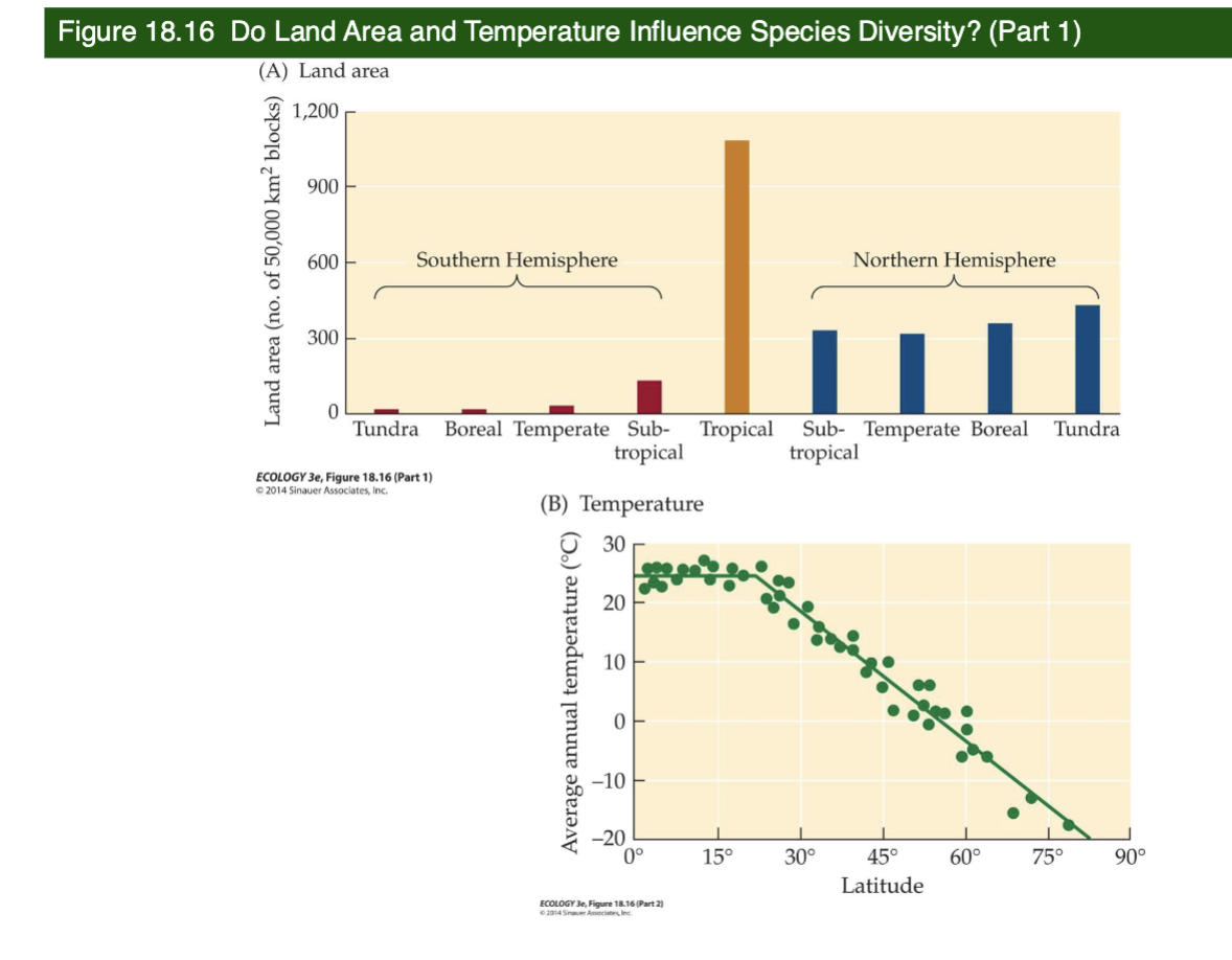
Explain Figure 18.16 — Michael Rosenzweig: Do Land Area and Temperature Influence Species Diversity?

• John Terborgh and Michael Rosenzweig proposed that terrestrial species diversity is highest in the tropics because the tropics have the largest land area (Figure 18.15A). Rosenzweig calculated that the region between 26° Nand S has 2.5 times more land area that any other latitude range on Earth. This makes intuitive sense, given that this latitude range is at the middle, and thus at the widest part, of the planet.

• Equally interesting are data showing that this very large area is also the most thermally homogeneous region on Earth (Figure 18.158). A plot of average annual temperature against latitude by Terborgh showed that land temperatures are remarkably uniform over a wide area between 25°N and S, but then drop off rapidly at higher latitudes.

Rosenzweig suggested that 2 two factors combine to decrease extinction rates and increase speciation rates in tropical regions

1. By increasing the population sizes of species (assuming that their densities are the same worldwide), and thus decreasing their risk of extinction due to chance events, and

2. By increasing the geographic ranges of species, and thus decreasing their chances of extinction by spreading the risk over a larger geographic area

• He further suggested that speciation should increase in larger areas because species should have larger geographic ranges, and thus should have a greater chance of reproductive isolation of population

2. Species diversification time

• The tropics are thought to have been more climatically stable over time, and species have had more time to evolve.

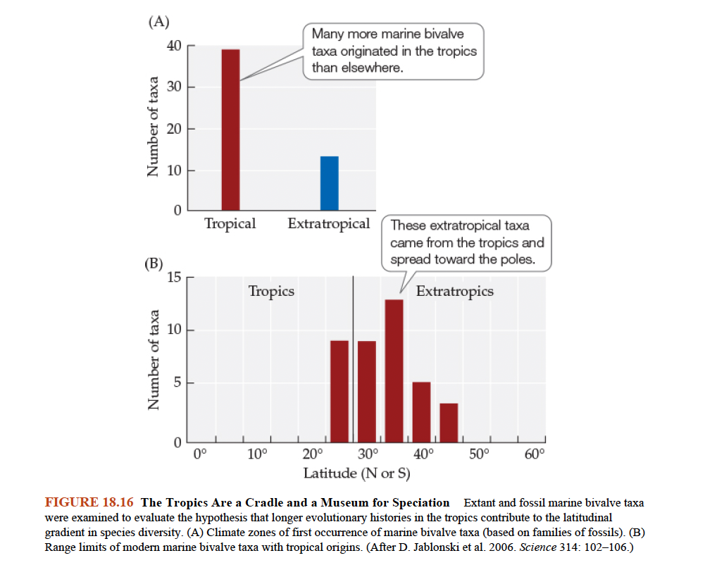
Figure 18.6- The Tropics Are a Cradle and a Museum for Speciation Extant

Jablonski et al. (2006)

• The tropics may serve as a cradle - species originate in there and to other regions

• Found that the majority of extant marine bivalve taxa originated in the tropics and spread toward the poles but without losing their tropical presence

• If extinction rates in the tropics are low, then species that diversify there will tend to stay there

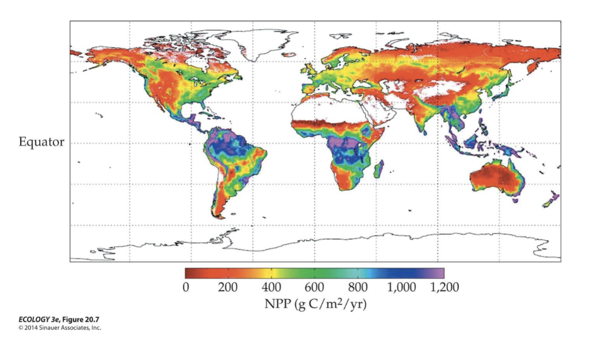
3. Productivity or Carrying Capacity

• Terrestrial productivity is highest in the tropics.

• High productivity promotes large population sizes because carrying capacity is larger.

• Higher productivity leads to lower extinction rates, greater coexistence, and overall higher species richness.

• Productivity could also explain the reverse pattern seen in sea birds.

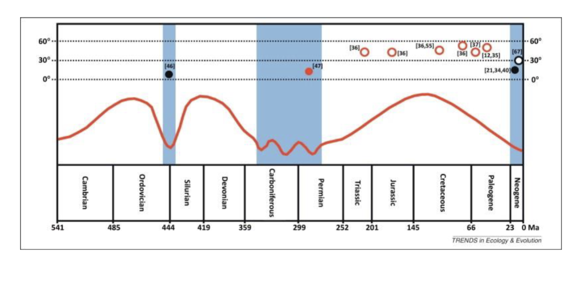
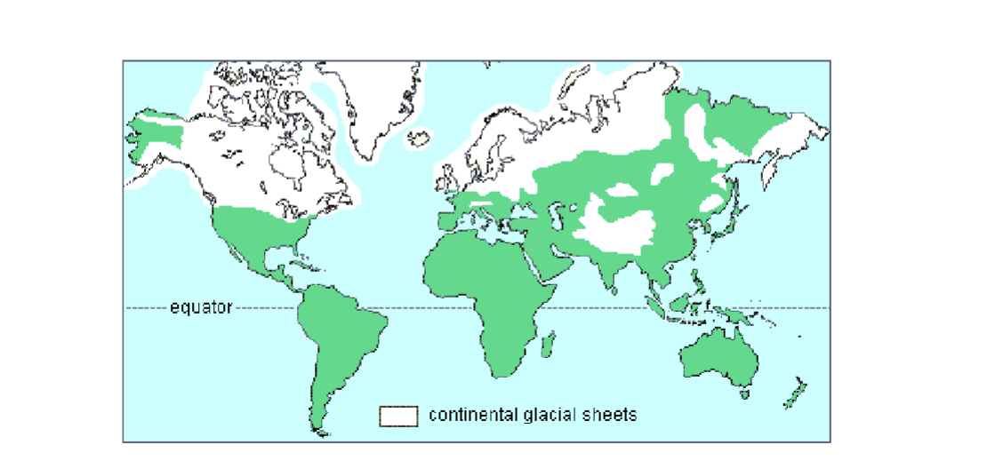
Mannion and colleagues (2014) looked at…

the fossil record to characterize species diversity by latitude across geological time.

What does the image Mannion deduce?

• Used the fossil record and fluctuations in past global temperatures as a window into past latitudinal and species diversity gradients and their potential causes.

• Their analysis showed that a tropical peak in species diversity has not been a universal pattern but has been restricted to particular intervals of time throughout the Phanerozoic when the Earth experienced colder, "icehouse" conditions they found that during warmer, "greenhouse" conditions,

• Species diversity peaked in temperate latitudes, exhibiting a more unimodal relationship. These switches from temperate to tropical peaks in species diversity corresponded to transitions in greenhouse to icehouse climate conditions, lending support for the notion that polar to temperate glaciations could drive species to the tropics where extinctions would be lower.

Regional differences in species diversity are influenced by area and distance, which determine…

the balance between immigration and extinction rates.

An important concept in biogeography is…

the species– area relationship

Species– area relationship

species richness increases with area sampled.

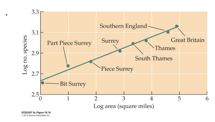
H.C. Watson plotted first species-area relationship, using plants in the Great Britain...in 1859

• Study: Plotted species richness of plants vs. area size in Great Britain.

• Findings:

  • Species richness increased with area sampled, showing a species–area relationship.

• Importance:

  • Laid the foundation for understanding how area affects biodiversity.

  • Proved that bigger areas support more species

Species–area curves plots…

species richness (S) of a sample against area (A).

The relationship between S and A is estimated by linear regression formula:

S= zA + c

Components of Species–area curves plot formula

S= Species richness
A= Area

z= slope

c= y-intercept

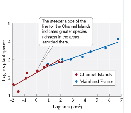
Ecological Toolkit 18.1, Figure A Species–Area Relationships of Island versus Mainland Areas (Part 2)

• The figure shows species–area curves for plants on the Channel Islands (off the coast of France) and on the French mainland (Williams 1964).

• An important characteristic of species–area curves is evident in this figure: the steeper the slope of the line (i.e., the greater the z value), the greater the difference in species richness among the sampling areas.

• The Channel Islands have a much steeper slope than the French mainland areas

• Species–area curves for plant species on the Channel Islands and in mainland France show that the slope of a linear regression equation (z) is greater for the islands than for the mainland areas.

Islands” are really useful for studying…

species-area relationships

An island can be a…

any kind of isolated area surrounded by dissimilar habitat (matrix habitat).

Habitat fragments, such as in the Amazon forest, can be considered as…

islands

All display the same basic pattern

large islands have more species than small islands.

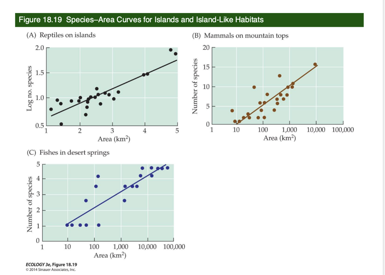
What does Figure 18.19- Species–Area Curves for Islands and Island-Like Habitats show?

• Species–area curves plotted for (A) reptiles on Caribbean islands, (B) mammals on mountaintops in the American Southwest, and (C) fishes living in desert springs in Australia all show a positive relationship between area and species richness.

• Species richness increases with area across many types of isolated habitats — not just true islands.

• Larger areas provide more habitat types, more resources, and lower extinction risks, allowing more species to persist.

• Isolation doesn't stop the area effect — mountains and springs (not just islands) follow the same rule.

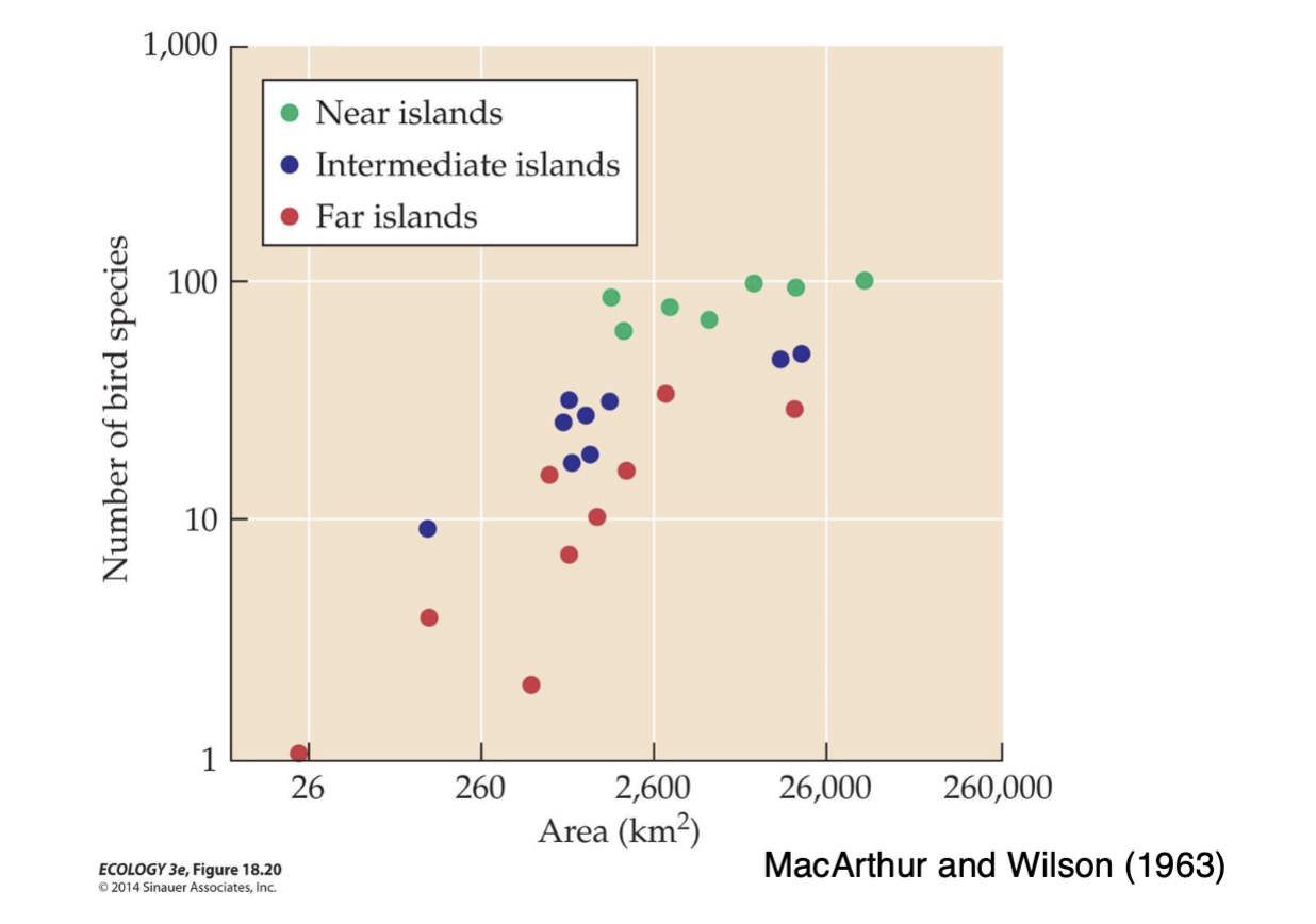
MacArthur and Wilson developed a
theoretical model…

The equilibrium theory of island biogeography

The equilibrium theory of island biogeography

The number of species on an island depends on a balance between immigration or dispersal rates and extinction rates.

The equilibrium theory of island biogeography effects on species richness

• Larger islands have more species because they have lower extinction rates (more habitat, larger populations).

• Islands closer to the mainland have more species because they have higher immigration rates (easier to reach).

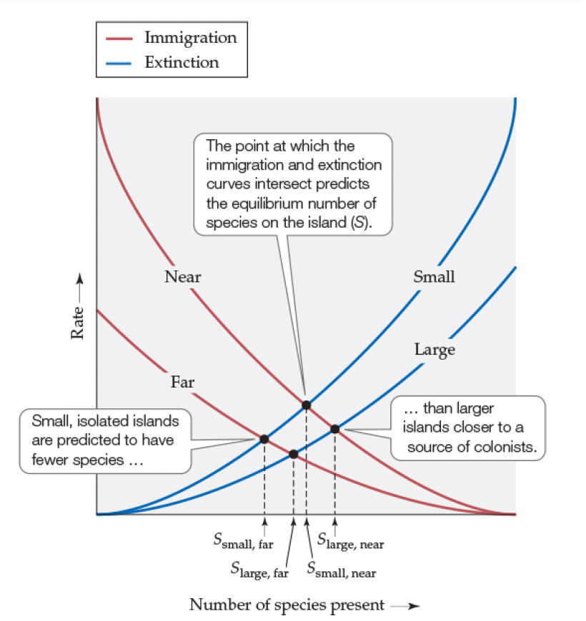
Explain this figure 18.21- The equilibrium Theory of Island Biogeography:

Small island ; Far Island Species Richness

Fewest species

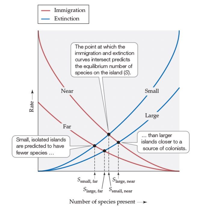
Explain this figure 18.21- The equilibrium Theory of Island Biogeography:

Large, far island

More Species than small-far, but still limited by distance

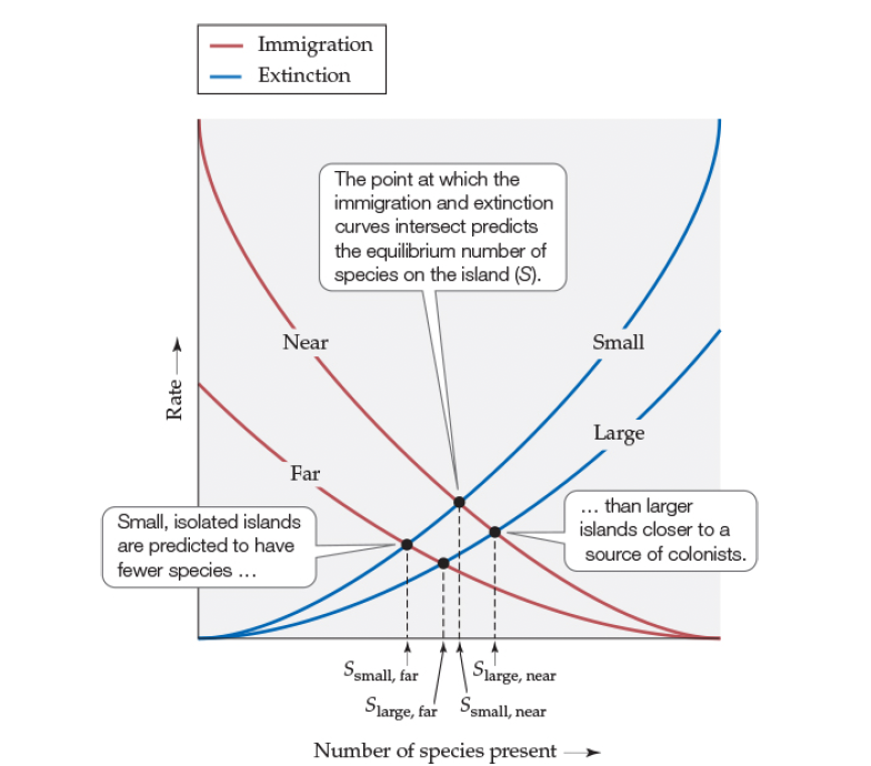
Explain this figure 18.21- The equilibrium Theory of Island Biogeography:

Small, near island

More species than distant islands, but limited by small size

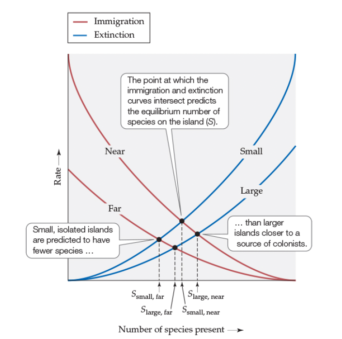
Explain this figure 18.21- The equilibrium Theory of Island Biogeography:

Large, near island

Most species overall

Why does immigration decrease as species richness increases?

As more species already live on the island:

• There are fewer new species left on the mainland that haven’t already colonized.

• Most of the potential colonists are already present, so the chance of a new species arriving and being new becomes lower.

In short:

• Fewer new species are available to immigrate as the island fills up.

Why does extinction increase as species richness increases?

As more species occupy the island:

• Competition for resources (like food, space) becomes stronger.

• Predation may increase (more predator species arrive).

• Population sizes of individual species shrink because they have to share limited resources.

Smaller populations are more vulnerable to:

• Random events (like storms, drought)

• Competition and predation

• Inbreeding and disease

In short:

• More species = more competition and smaller, weaker populations, so extinction risk rises.

MacArthur Wilson Experiment

1. Island Size Affects Extinction

• Small islands:

  • Have higher extinction rates.

  • Fewer resources and space → species populations are smaller → species are more likely to die out.

• Large islands:

  • Have lower extinction rates because they can support bigger, more stable populations.

2. Distance Affects Immigration

• Islands close to the mainland:

  • Have higher immigration rates (easier for species to get there).

• Islands far from the mainland:

  • Have lower immigration rates (harder for species to reach).

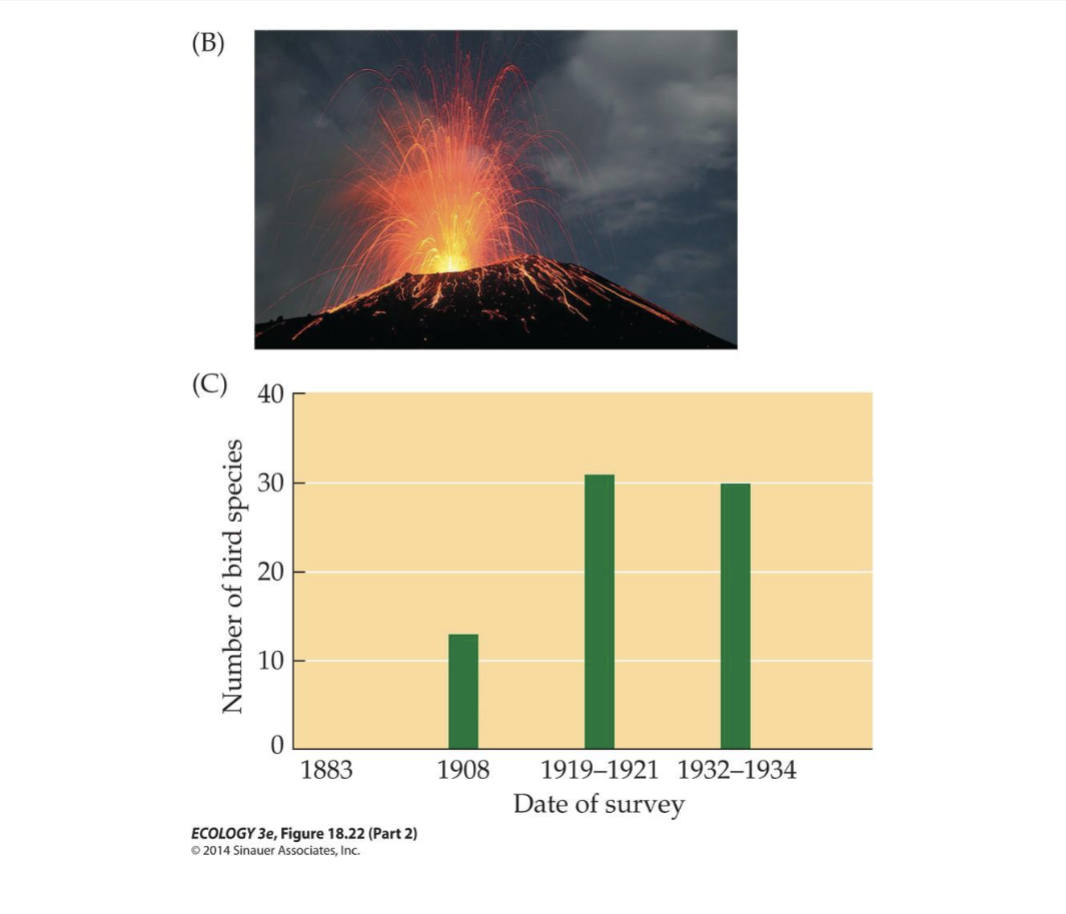
Testing the Theory with Krakatau:

• Krakatau (a volcanic island) erupted in 1883 and was wiped clean of life.

• After the eruption, plants and animals started recolonizing the island within a year.

• Wilson and MacArthur:

  • Collected data from three surveys over time.

  • Predicted Krakatau would reach about 30 bird species at equilibrium, with a low turnover (only 1 species changing at a time).

What they found:

• The number of bird species did stabilize around 30 species — matching their prediction! ✅

• However, the turnover rate was higher (about 5 species changing) — meaning species came and went more than expected.