One-way repeated measures ANOVA

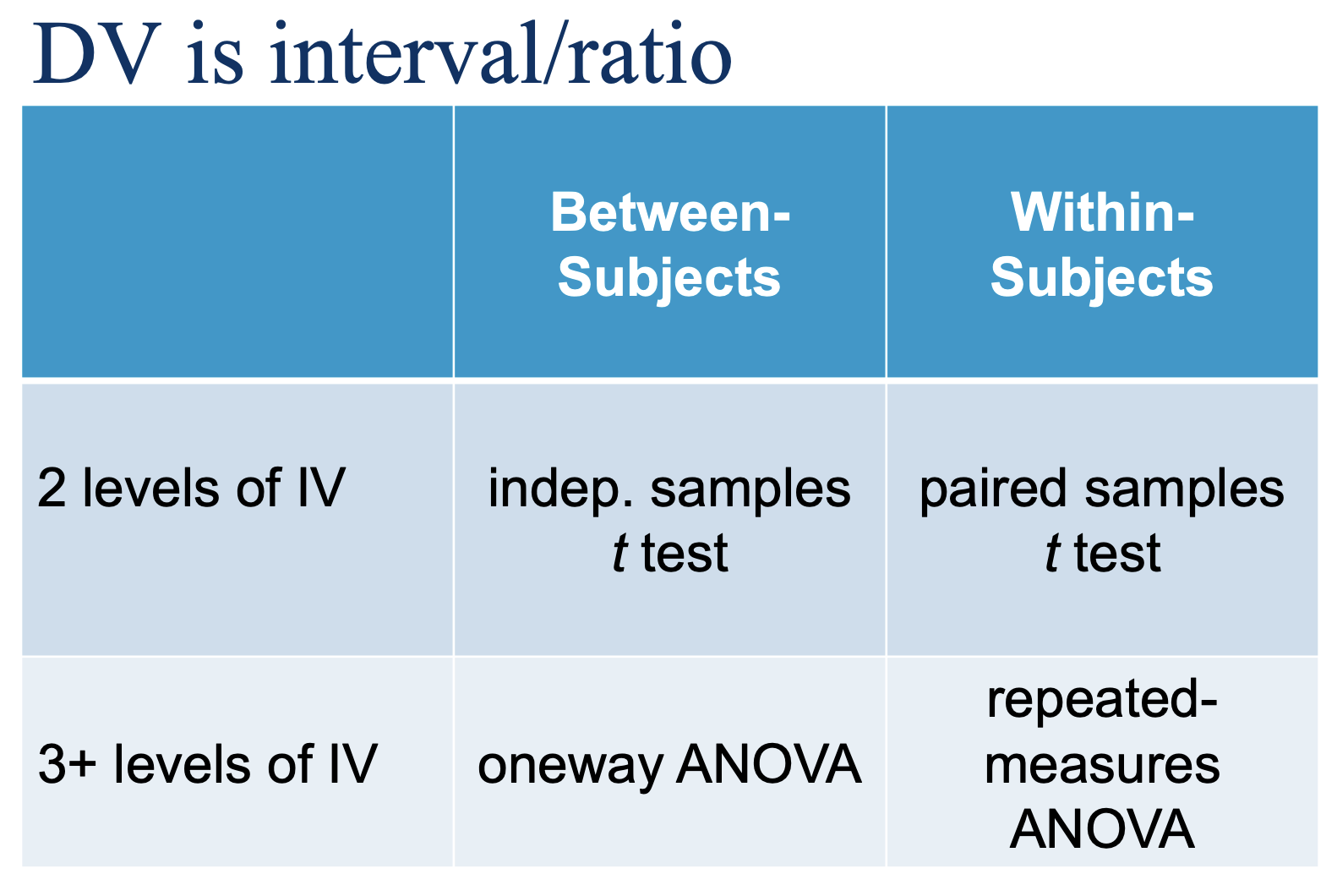
2 t-tests & 2 ANOVAS (fill out table); DV is…

WHEN do we use it?

• Interval or ratio DV

• Within-subjects (or matched) IV

• IV has 3 or more levels

WHY do we use it?

Rather than multiple correlated groups t tests?

• To avoid inflating Type I error rate (same reason as for one-way between-subjects ANOVA)

• A single F test keeps alpha @ .05

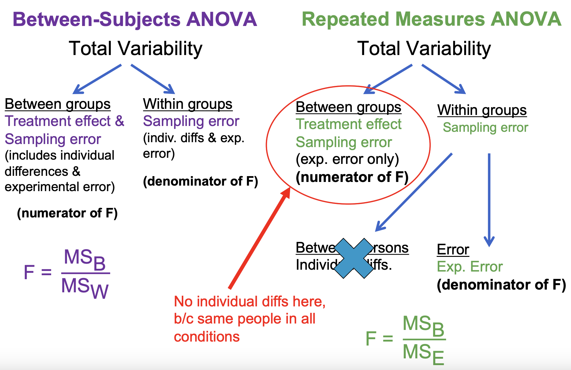
Logic of Between-Subjects vs. Repeated Measures ANOVA

Between-Subjects ANOVA

• Total Variability

  • Between groups: Treatment effect & Sampling error (includes individual differences & experimental error); numerator of F

  • Within groups: Sampling error (individual differences & experimental error); denominator of F

  • F = MSB (tells us why people are different across groups) / MSW (tells us why people are different within their group)

Repeated Measures ANOVA

• Total Variability

  • Between groups: Treatment effect & Sampling error (experimental error only); numerator of F; no individual diffs here, b/c same people in all conditions

  • Within groups: Sampling Error

    • Between persons: individual differences REMOVED

    • Error: Experimental Error (denominator of F)

  • F = MSB/MSE

Part 1: focus on individual differences BETWEEN groups — what is different with rmANOVA:

We will not have individual differences in the between group component, because participants are no longer going to differ ACROSS CONDITIONS

Part 2: focus on individual differences WITHIN groups — what is different with rmANOVA:

Here is the really key piece, and also includes how we are going to do the actual ANOVA test…

There is still variability from person to person WITHIN a group, but because we now have a way to calculate a measure of variability PER PERSON, we can use that knowledge to separate WITHIN group variability into two components: between persons and experimental error.

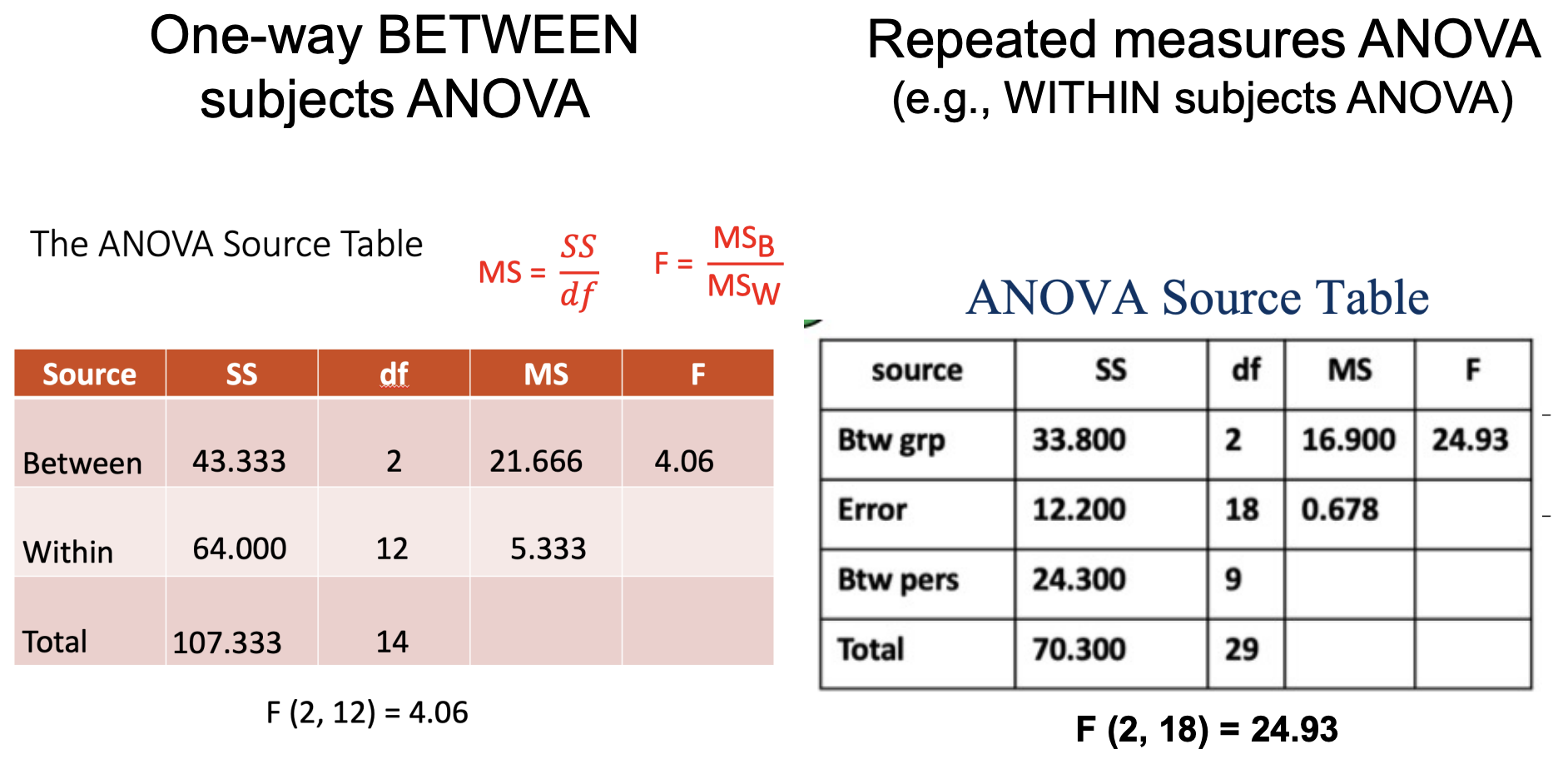
Comparing the ANOVA Source Tables

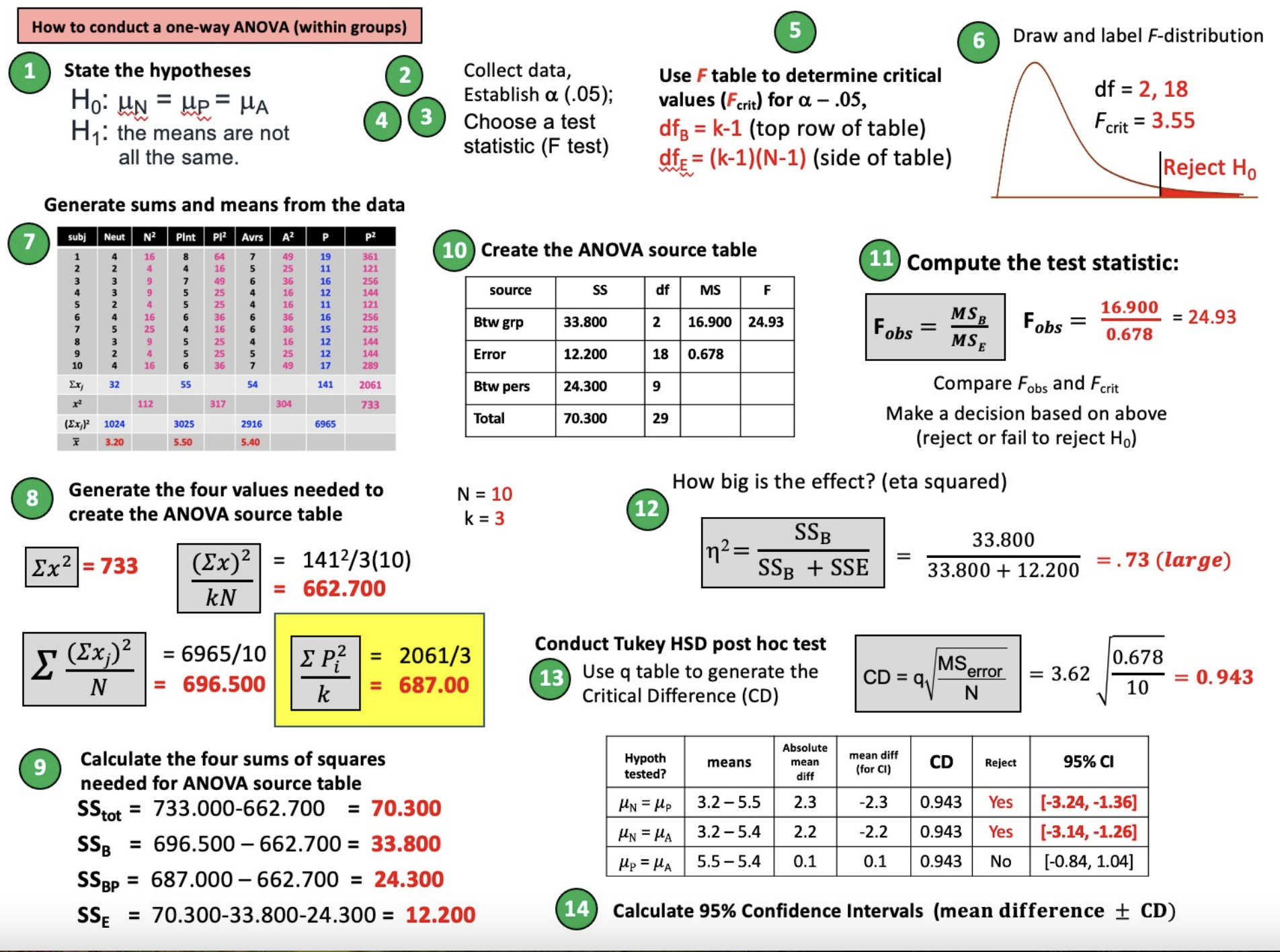
Steps in Hypothesis Testing

1. Establish H0 & H1

   • H0: µp = µa = µn (all population means are the same; there is no variance among the pop. means)

   • H1: The three population means are not all equal; there IS variance among the population means

   • note: n = N in repeated measures

2. Collect data

3. Characterize the sampling distribution (F) and determine the critical value from table

4. Calculate test statistic (F)

5. Make decision to reject or fail to reject H0

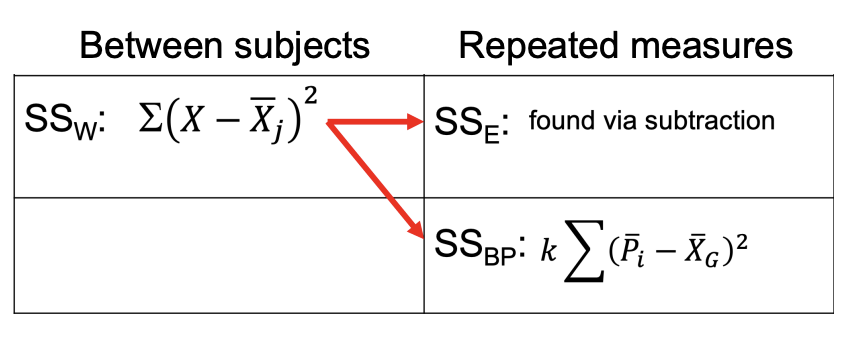
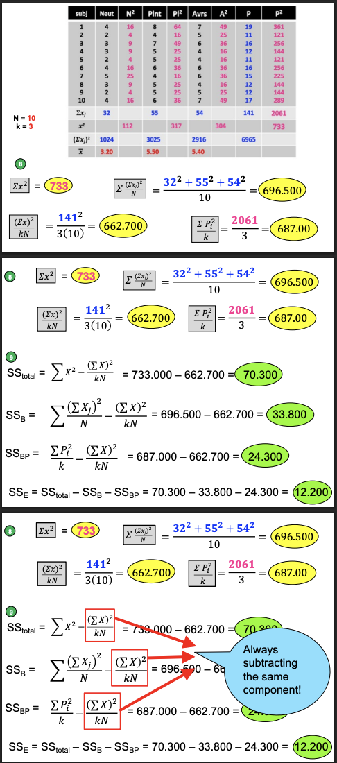
Comparing Definitional Formulas:

SST & SSB are the same; SSW split into:

• SSE: found via subtraction

• SSBP

• The SSW variability that you are familiar with calculating is still important. But, we get to partition SSW into two parts by calculating a measure of variability for EACH PERSON (SSBP). Then, we can exclude that SSBP when we calculate F ratio, which is F = MSB/MSE

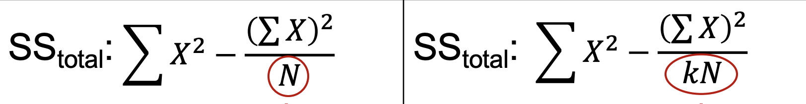
Comparing Computational Formulas: SST

Denominator: from N to kN— both of these represent the total number of observations in the data set

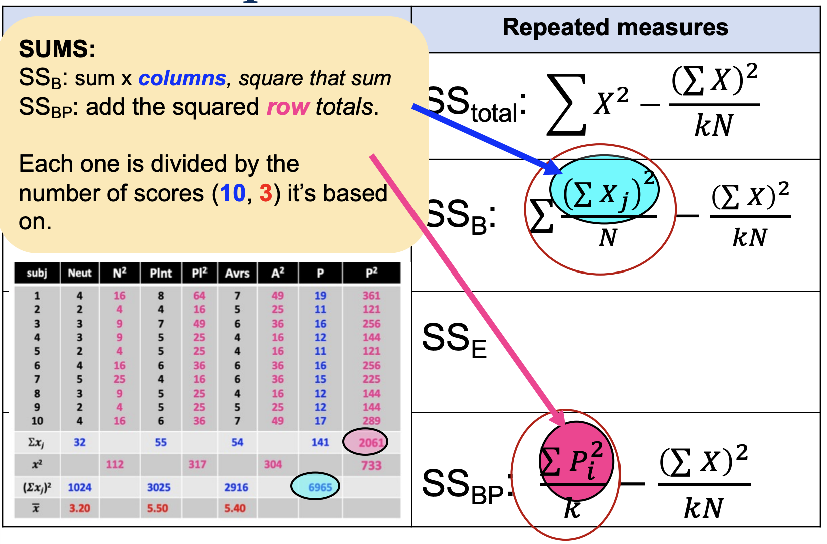
Comparing Computational Formulas: SSB & SSBP

SSB: sum of x columns, square that sum

SSBP: add the squared row columns

Each one is divided by the # of scores (10, 3) it’s based on

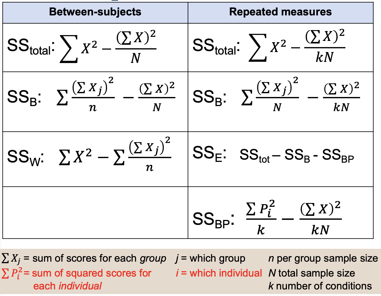
Computational Formulas, denote ∑Xj, ∑Pi², j, i, n, N, k

Degrees of Freedom total, between groups, error, & between persons

kN - 1

k - 1

(k - 1)(N - 1)

N - 1

Let’s compute our SS!

PEMDAS

How to conduct a one-way ANOVA (within groups)

How is P different from the D we calculated for the paired-samples t test?

D removes effect of individual diffs. to create a “pure” treatment effect.

P removes the effect of treatment to get a “pure” measure of independent differences. We compute a SS for independent differences and then remove it.

D— removes individual differences, leaves a clean treatment effect

P— removes treatment effect; isolates person-to-person differences (used to reduce error)

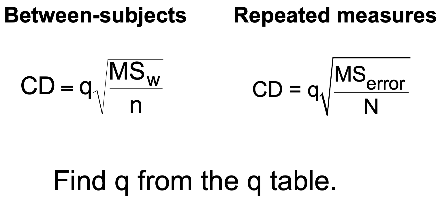
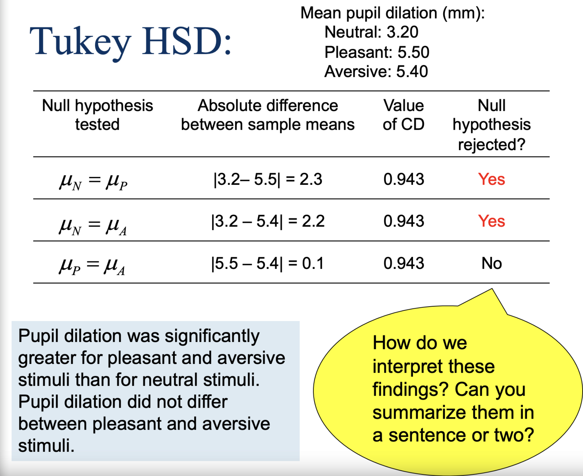
Post Hoc Analyses (Tukey HSD); computing the critical difference

Remember: range = k (number of groups), not dfbetween!

Tukey HSD

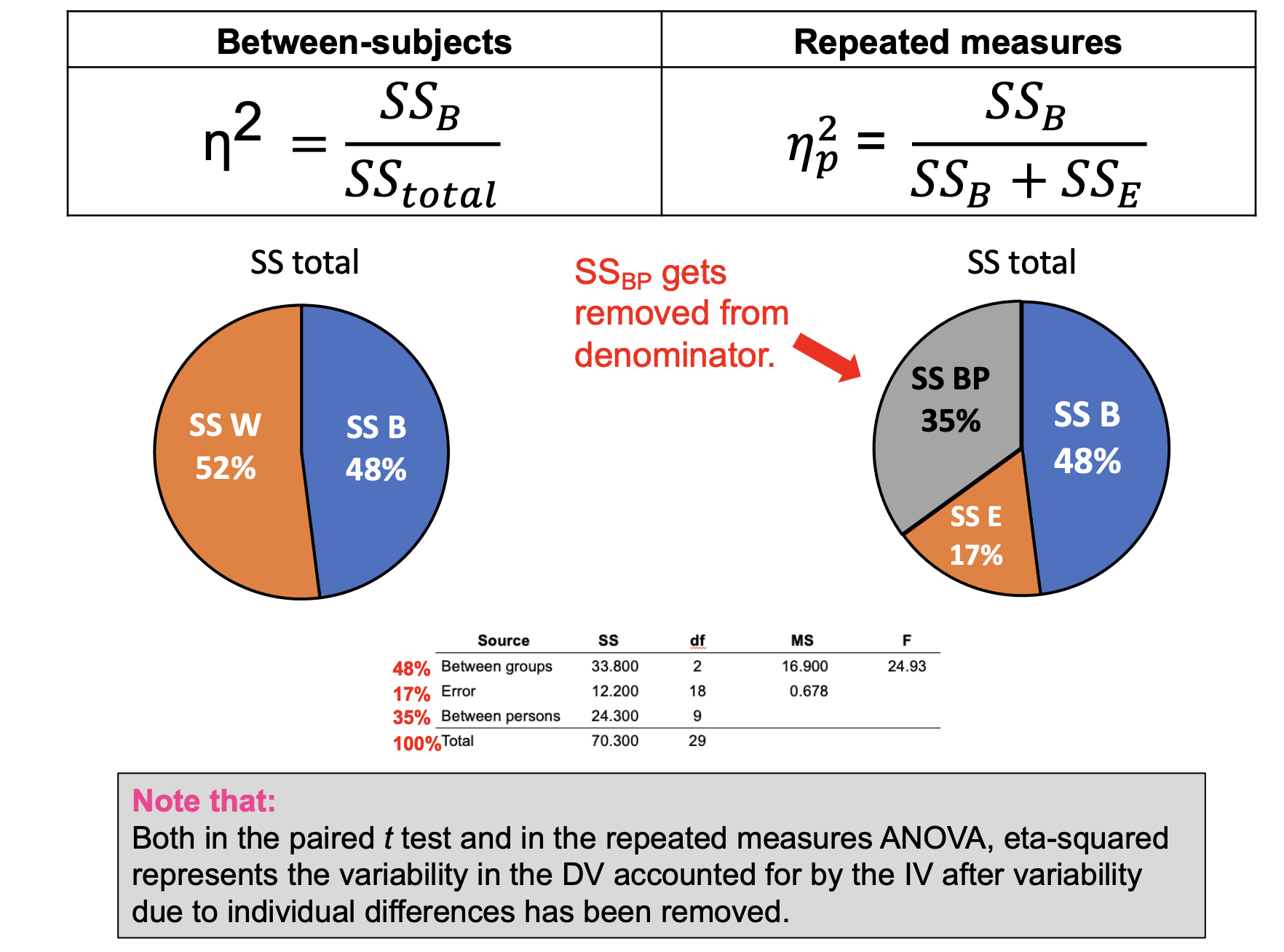
Strength of the relationship (partial eta-squared)

PSTT & RMA— eta-squared represents the variability in the DV accounted for by the IV after variability due to individual differences have been removed

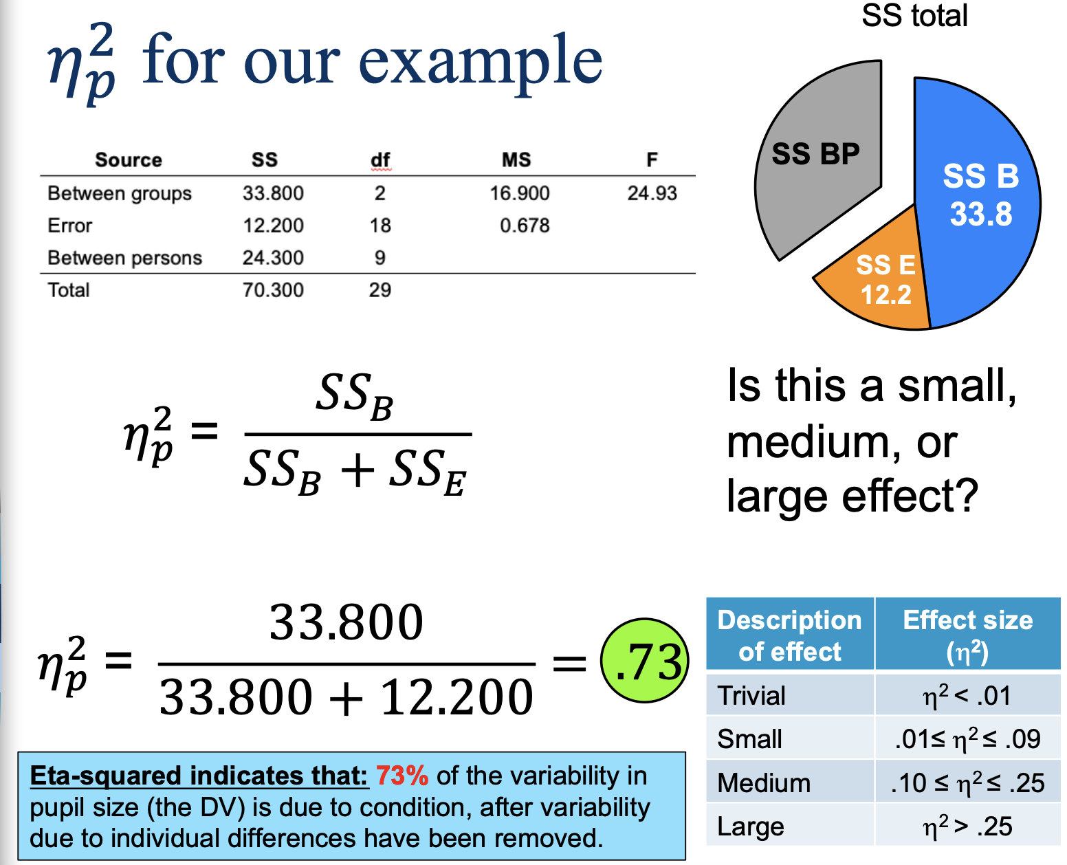
Partial eta-squared example

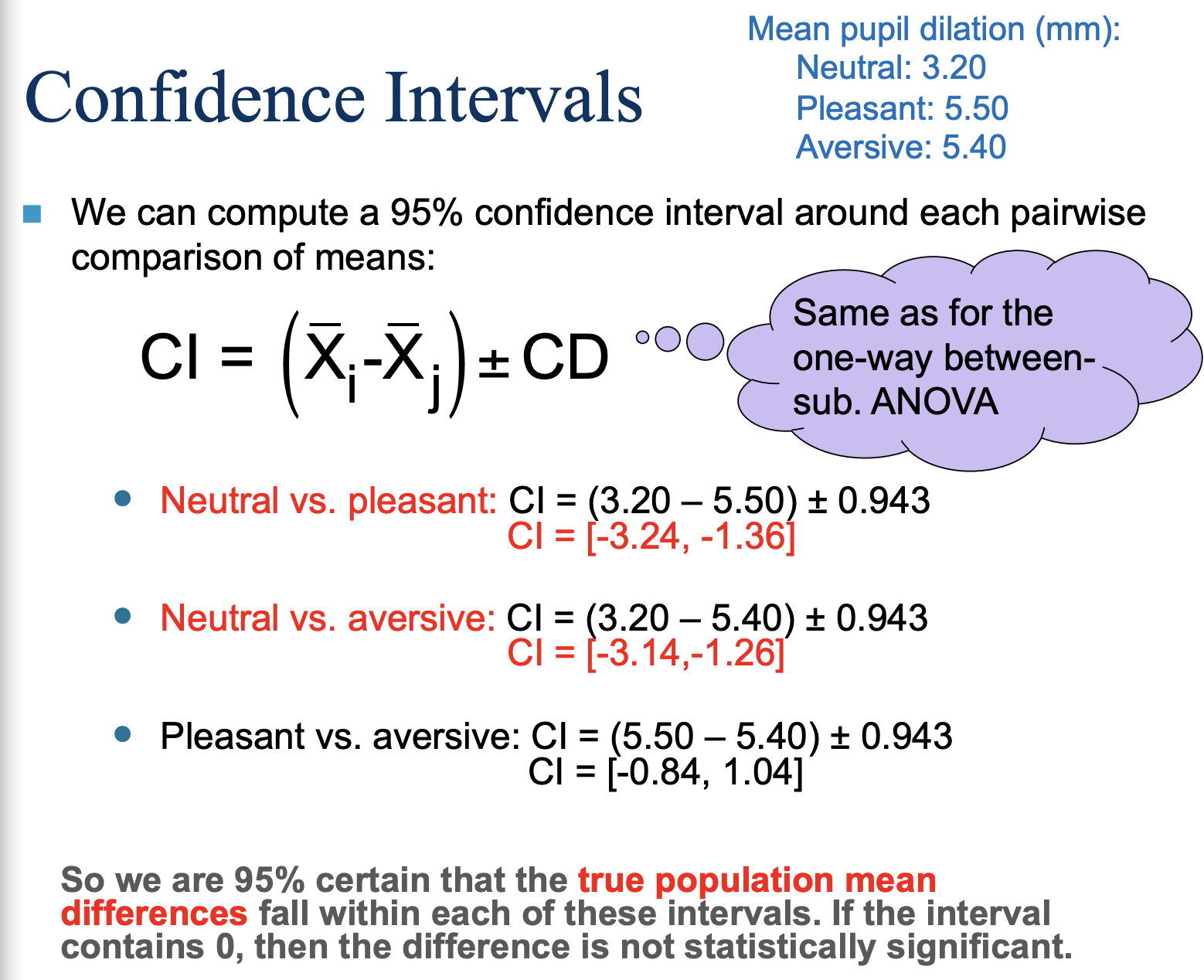
Confidence Intervals!

We are 95% certain that the true population mean differences fall within each of these intervals. If the interval contains 0, then the difference is not statistically significant.

Assumptions of the F test for repeated measures analyses

• Sample is independently and randomly selected from the population (i.e., rows are randomly selected).

• The scores in each population are normally distributed. (robust if N > 30)

• Populations have homogeneous variances.

• Sphericity

  • (test is not robust to violations of this assumption; Type I error (false positive) rate will increase if sphericity is violated)

  • Variance of population difference scores should be equal (for all pairs of differences)

  • Effect of the IV should be consistent across all participants (assumes everyone is equally affected by IV).

Explaining Sphercity

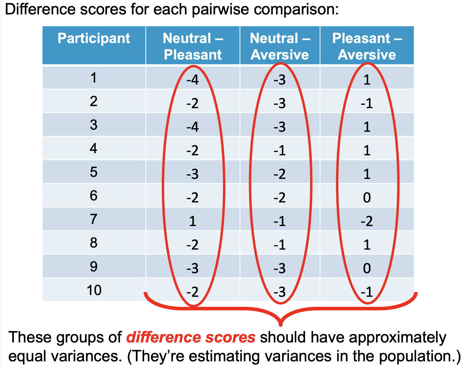
Difference scores for each pairwise comparison:

These groups of difference scores should have approximately equal variances (they’re estimating variances in the population).

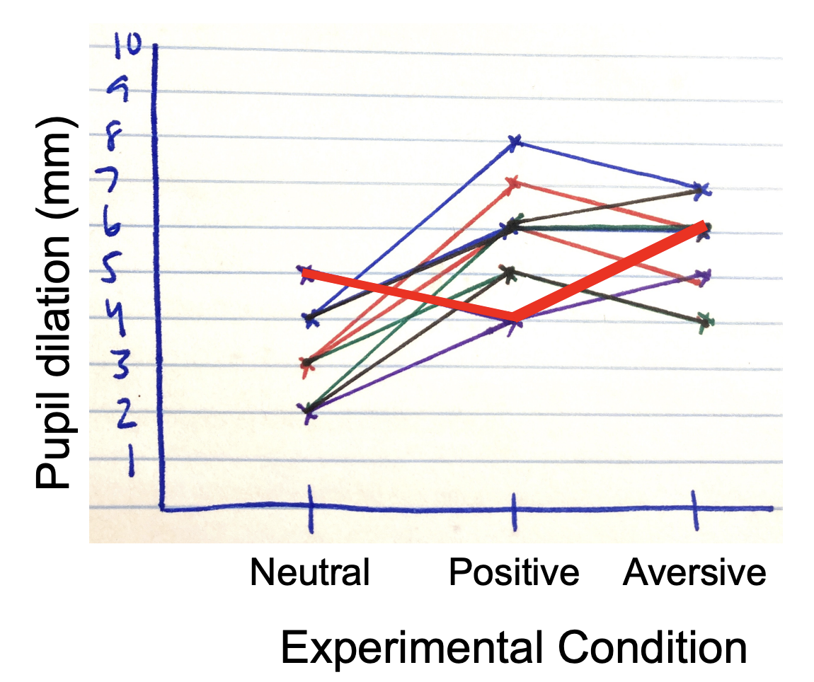
Visualizing Sphercity

Generally speaking, the effect of condition should be relatively similar for all participants.

Note:

By hand— Assume sphericity has NOT been violated! Just use a Tukey HSD test.

In SPSS:

• Mauchly test (BUT: The test under-detects sphericity violations in small samples and overdetects them in large samples).

• THM: Always assume sphericity has been violated and use one of two correction factors:

  • Huynh-Feldt epsilon

  • Greenhouse-Geisser epsilon

Rules for correction factors in SPSS

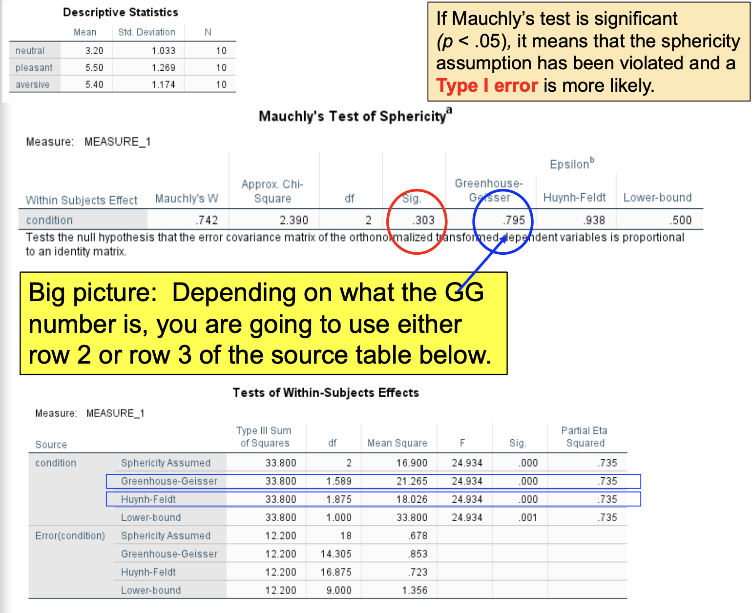
• If Maunchy’s test is significant (p < .05), it means that the sphericity assumption has been violated & Type I error is more likely

• Depending on what the GG number is, you are going to use either row 2 or row 3 of the source table below.

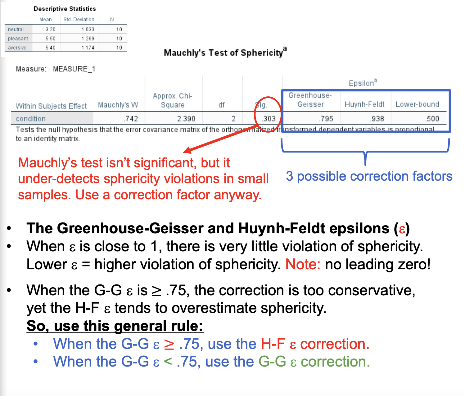
• Mauchly’s test isn’t significant, but it under-detects sphericity violations in small samples. Use a correction factor anyway.

  The Greenhouse-Geisser and Huynh-Feldt epsilons (e)

• When e is close to 1, there is very little violation of sphericity. Lower e = higher violation of sphericity. Note: no leading zero!

• When the GG is greater than or equal to .75, the correction is too conservative, yet the H-F e tends to overestimate sphericity

SO… we use this general rule:

• When the G-G e ≥ .75, we use the H-F e correction

• When the G-G e < .75, we use the G-G e correction

Rules for Correction Factors continued…

The correction simply adjusts the dfB and dferror by multiplying them by the epsilon. If sphericity hasn’t been violated, e is closer to 1 and won’t affect the df that much.

The epsilons are less than 1, so it makes the df smaller, resulting in a higher F critical value, making the F test more conservative (to correct for the possible Type I error).

You should still report F (2, 18) in your APA-style write-up. (Don’t report fractional df)

Notice that SPSS doesn’t provide dftotal or SStotal.

Be sure to report the partial eta-squared.

Rules for Correction Factors continued *2

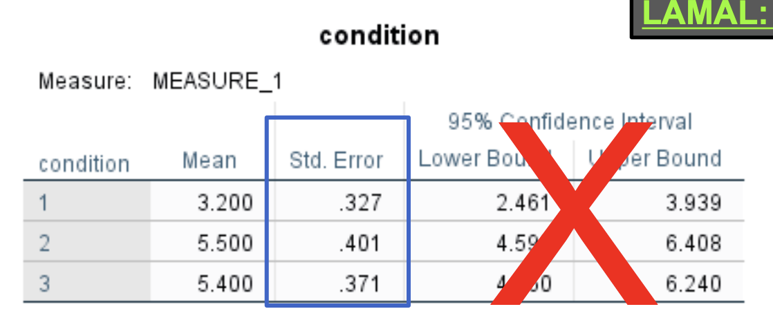
Selecting “EM Means” gives you the standard errors for each condition (useful if creating a bar graph).

Ignore these CIs; they are CIs around individual means, not around differences between means.

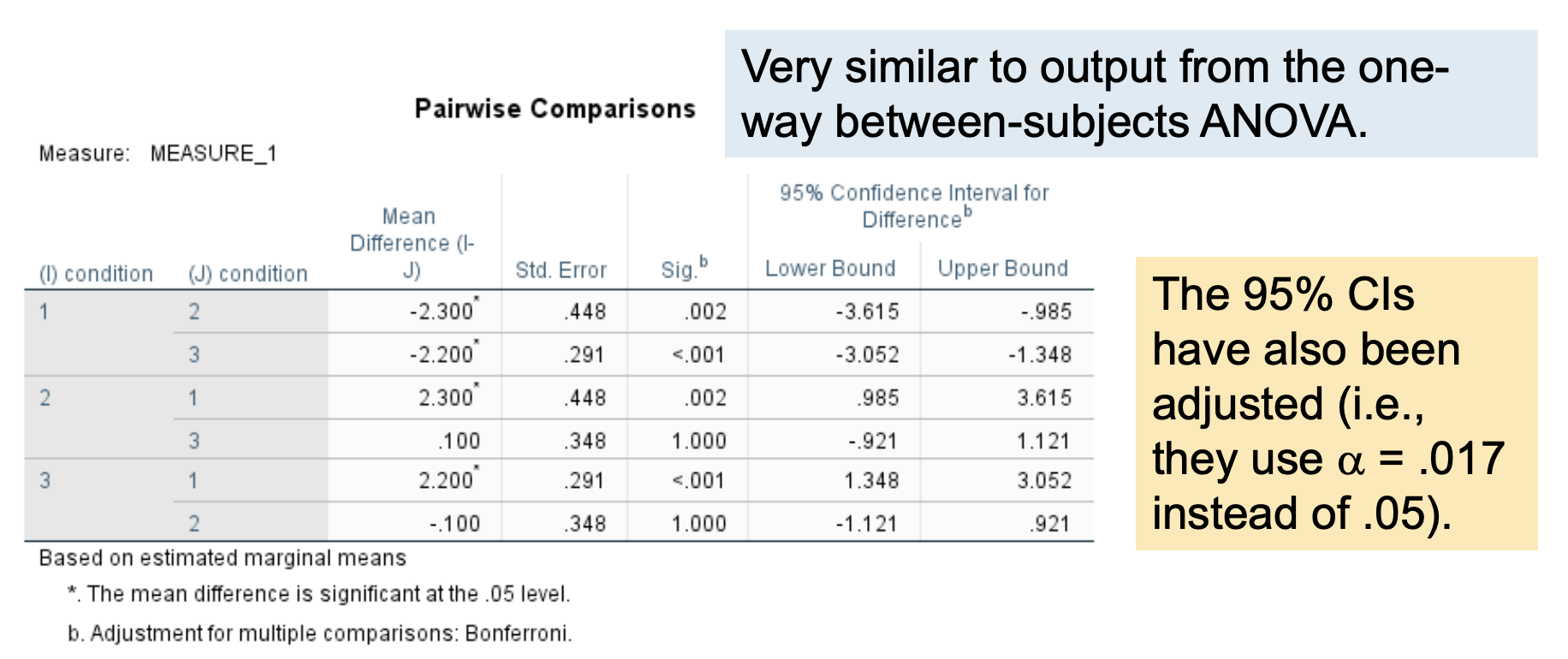
Understanding the nature of the effect: Pairwise comparisons with a Bonferroni correction

SPSS does not produce a Tukey HSD test for a repeated-measures ANOVA, because sphericity violations (which are common) make using the MSerror in the CD formula problematic.

Instead, pairwise comparisons (paired-samples t tests) are conducted using a Bonferroni procedure to control Type I error rate.

The Bonferroni procedure keeps the experimentwise a at .05 by adjusting the testwise a according to the # of comparisons.

Simply divide a by the # of pairwise comparisons:

• 3 conditions = 3 pairwise comparisons, so a = .05/3 = .017

• 4 conditions = 6 pairwise comparisons, so a = .05/6 = .008

These are just paired-samples t tests.

The original p value has been multiplied by the # of pairwise comparisons (in this case, 3). So you can compare the p here to .05. This is analogous to dividing a by 3.

The rest of the output can be ignored:

• Multivariate tests

• Tests of within-subjects contrasts

• Tests of between-subjects effects

Sample APA-style Results Section (using SPSS)

A one-way repeated measures ANOVA was conducted on pupil dilation (in mm) as a function of type of stimulus viewed (neutral, pleasant, or aversive). Mauchly’s test indicated that the assumption of sphericity was not violated, χ2 (2) = 2.39, p = .303, but because the test is highly sensitive to sample size, the degrees of freedom were still corrected using the Huynh-Feldt estimate of sphericity (e = .94). As hypothesized, pupil dilation was significantly related to type of stimulus, F(2, 18) = 24.93, p < .001, partial η2 = .79. Post-hoc pairwise comparisons using the Bonferroni correction indicated that, as hypothesized, average pupil dilation for neutral stimuli (M = 3.20, SD = 1.03) was significantly smaller than for both pleasant (M = 5.50, SD = 1.27), p = .002; 95% CI [-3.62, -0.98] and aversive stimuli (M = 5.40, SD = 1.17), p < .001; 95% CI [-3.05, -1.35]. Average pupil dilation for pleasant and aversive stimuli did not significantly differ, p = 1.00; 95% CI [-0.92, 1.12].

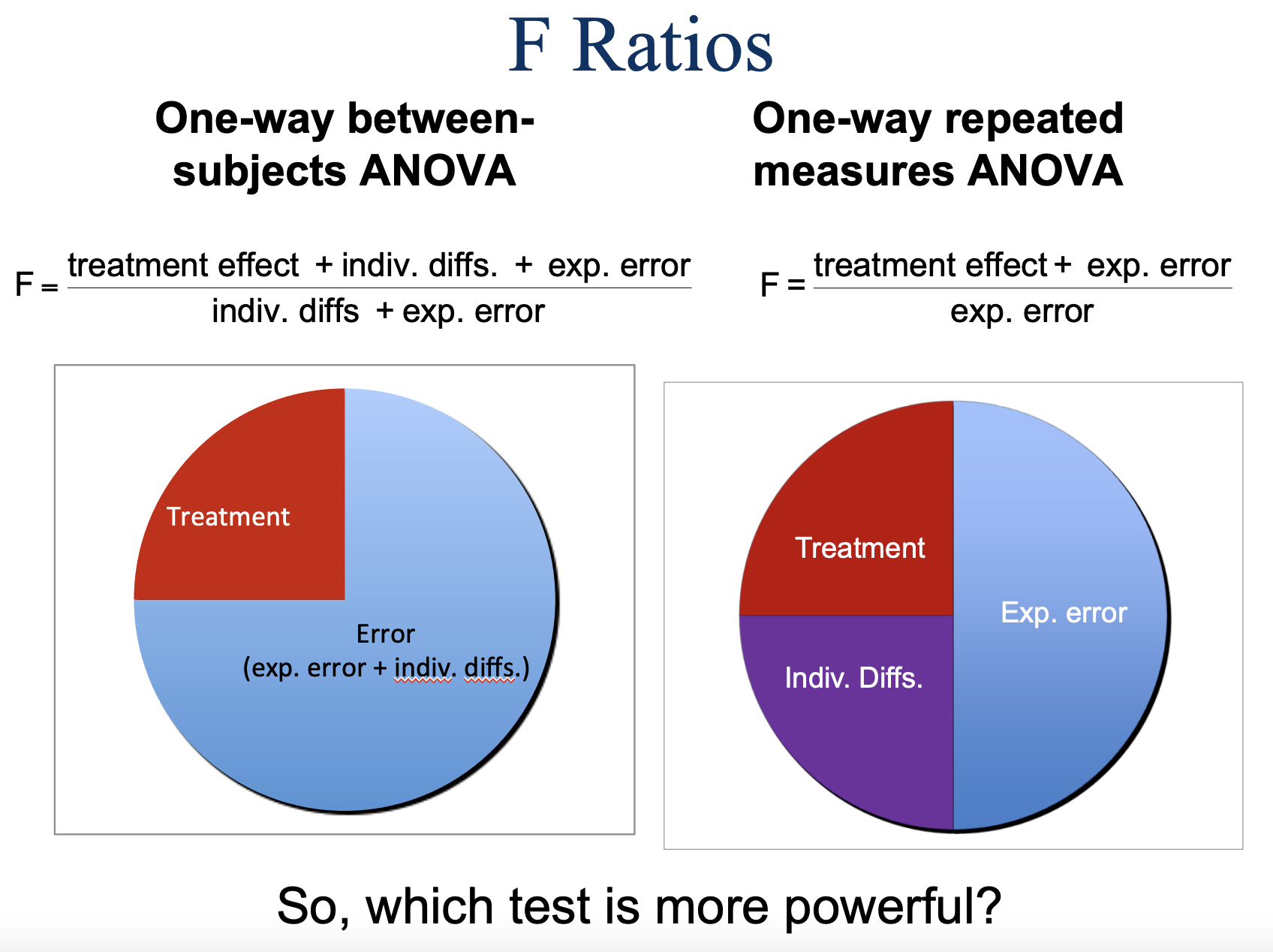
Visualizing F ratios

reduces variability (noise) by using the same participants in all conditions; each participant acts as their own control, removing between-persons V / increasing sensitivity to real effects