Test #2 Content: ENVSOCTY 3GV3 - Advanced Vector GIS

Facilities - Feature Class Input Properties (Network Analysis)

• FacilityType

  • 0 = Candidate

  • 1 = Required

  • 2 = Competitor

  • 3 = Chosen

• Weight

  • Relative weighting of a facility according to its attractiveness, desirability, importance, etc.

• Capacity

  • How much weighted demand a facility is capable of supplying

• CurbApproach

  • Direction of travel when arriving at or departing from facility

Facilities - Feature Class Output Properties (Network Analysis)

• DemandCount

  • # of demand points allocated to a facility

• DemandWeight

  • Sum of weights of all demand points allocated to a facility

• Total_[Cost]

  • Sum of the network costs between a facility and the demand points allocated to it

• TotalWeighted_[Cost]

  • Cumulative weighted cost for a facility

Demand - Points Feature Class Input Properties (Network Analysis)

• GroupName

  • Name of the group a demand point is part of

• Weight

  • Relative weighting of demand point

• ImpedanceTransformation

  • Overrides the network analysis layer’s impedance transformation value

  • Linear, power, exponential

• ImpedanceParameter

  • Overrides the network analysis layer’s impedance parameter value

• Cutoff_[Cost]

  • Overrides the network analysis layer’s Cutoff value

  • Ex; 5 minute cutoff (nobody going to demand point if greater than 5 min away)

• CurbApproach

  • Direction of travel when arriving or departing from a demand point

Demand - Points Feature Class Output Properties (Network Analysis)

• FacilityID

  • Object ID of the facility the demand point is allocated to

    • Null values indicates that the demand point was not allocated to facility or was to more than one facility

• AllocatedWeight

  • Null = demand point was not assigned to a facility (outside of cutoff)

  • 0 = demand point is only assigned to competing facilities

  • + Value = amount of demand assigned to chose and required facilities

Lines Feature Class (Network Analysis)

• Output only class that contains line features that connect demand points to the facilities they are allocated to

• Represents shortest network path between a demand point and facility

Lines Feature Class Properties (Network Analysis)

• Name

  • Name of the line formatted such that the facility name and demand point name are listed in order they are visited

• FacilityID or DemandID

  • IDs of conencted features

• Weight

  • Weight assigned from a demand point to a facility

• TotalWeighted_[Cost]

  • Weighted cost of traveling between a demand point and facility

Point, line, and polygon barriers classes (Network Analysis)

• Serves to temporarily restrict or alter costs on parts of the network

  • Ex; flooding (polygon barrier)

• When a new network analysis layer is created, the classes are empty

• They are populated only when you add objects into them

  • Adding barriers not required

• Available in all network analysis layers

Impedance Transformation

• Function that transforms the cost of travel between demand and facilities

Types of Impedance Transformations

• Linear cost = impedance

• Power cost = impedance^b

• Exponential cost = e^{(b x impedance)}

Impedance Parameter (b)

• Parameter value set by user, which can emphasize near or distant locations

Ranges of Impedance Parameter (b)

• b > 1

  • Emphasizes distant locations (higher impedance costs for distant)

  • As value increases emphasis increases

• 0 < b < 1

  • Emphasizes nearby locations (higher impedance costs for nearby)

  • As value decreases emphasis increases

• ± values of b

  • Will result in the same solution

7 Location-Allocation Models

• Minimize weighted impedance (P-Median)

• Maximize coverage

• Maximize capacitated coverage

• Maximize coverage and minimize facilities

• Maximize attendance

• Maximize market share

• Target market share

Minimize Weighted Impedance Objective

• Given N candidate facilities and M demand points with weights. locate P facilities such that the sum of all weighted costs between demand points and solution facilities is minimized

Minimize Weighted Impedance Examples

• Private sector: Warehouses

  • Optimal locations for a warehouse which will minimize a cost

• Public sector: libraries, health clinics, etc.

Minimize Weighted Impedance Handling of Demand

• If an impedance cutoff is set, any demand outside all the facilities’ impedance cutoffs is not allocated

• A demand point inside the impedance cutoff of one facility has all its demand weight allocated to that facility (‘all or nothing’)

• A demand point inside the impedance cutoff of 2 or more facilities has all its demand weight allocated to the nearest facility only

Maximize Coverage Objective

• Given N candidate facilities and M demand points with weights, locate P facilities such that the number of demand points covered by solution facilities is maximized within an impedance cutoff

• Covering as many demand points as possible!

Maximize Coverage Examples

• Public sector

  • Emergency response facilities like fire station, police stations, etc.

• Private sector

  • Delivery service facilities

    • Pizza delivery

Maximize Coverage Handling of Demand

• Any demand point outside all the facilities impedance cutoffs is not allocated

• A demand point inside the impedance cutoff of one facility has all its demand weight allocated to that facility

• A demand point inside the impedance cutoff of 2 or more facilities has all its demand weight allocated to nearest facility only

*Demand is handled the same way as minimize impedance

Maximize Capacitated Coverage Objective

• Given N candidate facilities and M demand points with weights, locate P facilities such that the number of demand points covered by solution facilities is maximized and the weighted demand allocated to a facility does not exceed the facility’s capacity

Maximize Capacitated Coverage Examples

• Public sector;

  • Facilities that are built with defined capacities like hospitals or schools

Maximize Capacitated Coverage Handling of Demand

• If an impedance cutoff is specified, any demand point outside all the facilities impedance cutoffs is not allocated

• An allocated demand point has all or none of its demand weight assigned to a facility—demand is not apportioned

• If the total demand within the impedance cutoff of a facility is greater than the capacity of the facility then only the demand points that maximize total captured demand and minimize total weighted impedance are allocated

Maximize Coverage & Minimize Facilities Objective

• Given N candidate facilities and M demand points with weights, locate P facilities such that the number of demand points covered by solution facilities is maximized with an impedance coverage

• Additionally, the number of facilities required to cover demand is minimized

• Same as maximize coverage except solver chooses P

Maximize Coverage & Minimize Facilities Examples

• Same as maximize coverage when cost of building is not a factor

• Public sector;

  • School bus stops

    • Minimize # of bus stops but want to serve all demand points

Maximize Coverage & Minimize Facilities Handling of Demand

• Same as maximize coverage

Maximize Attendance Objective

• Given N candidate facilities and M demand points with weights, locate P facilities such that demand weight is maximized by the solution facilities while assuming that demand decreases in relation to the distance or travel time between facilities and demand points (distance decay)

Maximize Attendance Examples

• Private sector

  • Retailers, restaurants, coffee shops

• Public sector

  • Transit stops

Maximize Attendance Handling of Demand

• Demand outside the impedance cutoff of all facilities is not allocated to any facility

• When a demand point is inside the impedance cutoff of one facility, its demand weight is partially allocated according to the cutoff and impedance transformation

• The weight of a demand point covered by more than one facility’s impedance cutoff is allocated only to nearest facility

Distance Decay

• Refers to the decrease in spatial interaction with distance from a location

• For Maximize Attendance, it is specified by an impedance transformation and parameter

  • Specification should be based on empirical information

Linear Decay Formula

• Demand = weight x (1 - (linear cost/cutoff))

• Equal weight with distance of facilities

Power Decay Formula

• Demand = weight x power cost

• High weight to nearby facilities

Exponential Decay Formula

• Demand = weight x exponential cost

• Very high weight to nearby facilities

Maximize Market Share Objective

• Given N candidate facilities and M demand points with weights, locate P facilities such that demand weight is maximized by the solution facilities in the presence of competitors

• Requires weights (relative measures of attraction) for candidate facilities as well as competitor facilities

• Uses a Huff Model

Maximize Market Share Examples

• Private sector

  • Same as Maximize Attendance providing you have access to weights of competitor facilities

  • Discount stores

Maximize Markey Share Handling Of Demand

• Demand outside the impedance cutoff of all facilities is not allocated to any facility

• A demand point inside the impedance cutoff of one facility has all its demand weight allocated to that facility

• A demand point inside the impedance cutoff of 2 or more facilities has all its demand weight allocated to the facilities that cover it. The weight is split among the facilities proportionally to the facilitys attractiveness and inversely proportional to the distance or travel time between the facility and demand point (Huff Model)

• Total market share is the sum of the weight of all demand points located on the network

  • Use the calculate captured market share

    • Percent of people going

Target Market Share Objective

• Given N candidate facilities and M demand points with weights, P facilities are located to capture a specific percentage of the total market share in the presence of competitors

  • Solver chooses the # of facilities for you

• Requires weights for candidate facilities as well as competitor facilities

• Uses a Huff Model

Target Market Share Examples

• Same as maximize attendance providing you have access to weights of competitor facilities

  • Discount stores

Target Market Share Handling of Demand

• Same as maximize market share

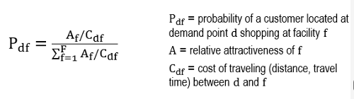
Huff Model

• Typically used to address the following question;

  • What is the likelihood that a customer will shop at a particular store given the presence of competitors?

• Demand is allocated to facilities within a cutoff as follows;

  • demand = weight x P

What models does B have no effect on?

• Maximize coverage

• Maximize capacitated coverage

• Maximize coverage & minimize facilities

How are the best sties selected (optimization)?

• Combinatorial problem

  • n choose p

    • n! / p!(n-p)!

• Typically not used for obvious reasons… very high values

How are the best sites selected (Vertex Substitution Heuristic)

1. Generate a random configuration of P facilities (initial solution)

2. Pick a candidate facility from the pool of remaining candidates

3. Calculate if candidate facility can be used to replace, one at time, each of the P facilities

4. Swap candidate facility with facility in P that yields the greatest improvement

5. Continue steps 2-4 until no further improvement is found

Vehicle Routing Problem

• Problems involve routing a fixed number of vehicles (routes), through a set of stops (orders) such that total travel cost (travel time, distance) is minimized, and vehicle capacity constraints are not violated

• Can be viewed as a fleet version of the traveling salesman problem

• Partitions stops among vehicles subject to capacity constraints and finds the shortest tour or route for the stops assigned to each vehicle

  • Tours start and end at a depot

  • Order in which stops are visited is determined

Service Area

• Problems involve assigning portions of a network to a location based-on predetermined criteria

Service Area - Public Sector Problems

• Locations are public sector facilities (fire stations, police stations, parks, hospitals, etc.)

• Criteria;

  • Ex; walking distance to schools, response times for emergency services

Service Area - Private Sector Problems

• Service areas are referred to as trade areas or market areas

• Locations are retail and commercial establishments

• Criteria are based on travel times or distances to locations

Service Area - Accessibility Problems

• Locations are typically residences (could be places like workplaces)

• Criteria are based on travel times or distances from locations

• Is intersected with opportunities to derive a type of accessibility known as cumulative opportunity ( adds up # of locations within that distance or time threshold)

What would you do if you want to associate every link in a network with its closest facility - Service Area Problem

• Set up artificially high cutoff values, that way all links would be allocated to nearest facility

Shortest Path

• Finds the least cost (travel time, distance) route connecting 2 locations on a network

Traveling salesman problem

• Finds the least cost (travel time, distance) route that visits a set of stops from a specified starting location on a network

• Route starts and ends at the same location

• Order in which intermediate stops are visited is determined

Route analysis layer options if intermediate stops are visited

• Use current

  • Preserves the sequence of stops

  • Finds best route given the order of steps

• Find best

  • Reorders the sequence of stops to find the shortest possible route

• Preserve first & last stop

  • Reorders intermediate steps to find shortest possible route

• Preserve first stop

  • Begins at the first stop with other stops being reordered to find the shortest possible route

• Preserve last stop

  • Ends at the last stop with other stops being reordered to find the shortest possible route

OD Cost Matrix

• Finds the least cost paths (travel time, distance), through a network from multiple origins to multiple destinations

• Instead of just solving 1 record it can solve thousands

• Options;

  • Number of destinations to find

  • Cutoff

• Output is typically input for some other form of analysis in which network cost is more appropriate than straight-line distance cost (like near tool)

• We are most interested in the table it creates

Closest Facility

• Solver computes best routes between network locations (like fires) and facilities (like fire stations) and for each location, selects the path with lowest cost (travel time, distance), thus identifying the closest facility

• Options;

  • Number of facilities to find

  • Direction(s)

  • Cutoff

• Solver can display best routes through the network and directions

• Can perform many analyses at once (such as multiple accidents)

OD Cost Matrix vs. Closest Facility

• Closest facility solver can be used to create an OD cost matrix, but it will take more time

  • Can generate true shapes of routes

  • Can generate directions

• OD cost matrix solver is designed to handle large M x N problems

  • Cannot generate true shapes of routes

  • Cannot generate directions

What is Location Analytics?

• Concerned with enriching business data with geography to gain insights into customer behavior that could lead to enhanced decisions

What industry is location intelligence the most important for?

• Telecommunications

Examples of Applications of Location Intelligence

• Finance

• Real estate

• Supply chain

• Risk

• Marketing

• Management

Spatial Data Sources

• Census and postal geography boundaries

• Locations of facilities

  • Own and competition

• Customer data

• Demographic data from Census or other survey

• Behavioral data (distance decay)

• Road networks

  • Ex; DMTI

• Market segmentation data

  • Ex; PRIZM or Tapestry

• Digital orthophotos or other remotely sensed data

• Terrain models

Business Data Sources

• Record keeping and management control

• Billings

• Services rendered

• Financial

• Inventory

• Customer accounts or status

• Orders

• Shipping manifests

Issues with Business Data

• Expensive

• Maintenance and integration with existing systems

  • Spatial techniques couple it with geographic coordinate system

• Data quality issues

  • Addresses may be partially incomplete

• Temporal issues

  • May change over time

    • Ex; sending flyers to wrong people

Dissemination Block

• Lowest level of geometry which you can obtain a few attributes about

Dissemination Area (DA)

• Smallest division for mapping, complete coverage of Canada

• These boundaries respect the boundaries of census subdivisions and census tracts

  • Generally follow roads, or natural features

• Normally contain 400-700 people to avoid data suppression

Census Tract (CT)

• Urban or rural neighborhood boundaries defined within CMA or CA

• 6,247 nationally

• Boundaries follow main streets and permanent + easily recognizable physical features

• Have populations between 2500-8000 people with average of 4000 people

• Have similar economic status and social living conditions at time of their creation

• Respect CMA, CA, and provincial boundaries

Census Subdivision (CSD)

• Municipalities or equivalent

  • Ex; towns, villages

  • 5,161 nationally

Census Division (CD)

• Group of neighboring municipalities joined together for the purposes of regional planning and managing common services

• 293 nationally

Census Metropolitan Area (CMA)

• Area consisting of one or more neighboring municipalities situated around a core with forward or reverse commuting

• Must have a total population of at least 100,00 of which 50,000 or more live in the core

• 41 nationally

• Hamilton’s includes Burlington and Grimsby

Census Data

• Conducted every 5 years in Canada

• 2 forms are

  • Short form (100% distributed)

  • Long form (25% random sample)

• Takes about 2 years from collection to release

  • Large scale statistics released first

  • DA released last

Census 2A

• 100% of population

• Population by age

• Sex

• Marital status

• Mother tongue

• Dwellings by tenure

• Structural type and size

• Family structure

• Number of children living arrangements

Census 2B

• 25% Random sample

• Population by home and official languages

• Ethnic origin

• Citizenship and place of birth

• Immigration status

• Religion

• Mobility status

  • If you have moved recently

  • Transportation (to work, etc.)

• Labor force

  • Full-time or part-time

• Occupation

• Industry

• Income

  • Used to be self-reported

• Households and dwellings by period of contruction

• Need for repairs

  • When was the household built?

CHASS

• Canadian census anlayser

• Open-access while on campus

Market Segmentation Data

• Involves identifying subgroups of people within a larger population such that each subgroup has similar needs or desires

• ‘Homogeneous group of consumers you can sell a product too’

Demographic Market Segmentation Data

• Method assumes that people’s values, interests, and attitudes can be traced back to demographic characteristics

• Typical segments might include (sociodemographic descriptions);

  • Millennials

  • Boomers

  • 2-parent households with 1 child under 5

  • Single women aged 18-34

  • Retired adults aged 50-69 who have an advanced degree

Geographic Market Segmentation Data

• Assumption is made that people’s values, interests, and attitudes can be traced to their geographic characteristics

  • ‘People who live close to each other, share similar characteristics’

• Typical segments might include;

  • People living in the downtown core

  • People living in rural areas

  • People living in drought, hurricane, or flood zones

Behavioral Market Segmentation Data

• What hobbies do they participate in? What products and services do they use and buy? What are their shopping routines?

• Typical segments might include;

  • People who grocery shop once per week and use at least 10 coupons each time

  • People who do most of their online shopping using a tablet or cell phone

  • People who use social networks at least 3 hours every day

Psychographic Market Segmentation Data

• Focuses on people’s attitudes, opinions, personality characteristics, life goals, social standing, and other more conceptual and flexible variables

• Segments might include;;

  • People who practice mindful thinking and believe in helping others achieve their goals

  • People who like to be alone and think each person should be responsible for themselves

  • Early adopters

What’s the segmentation data in Canada called and how many segments are there?

• PRIZM

• 67

Suitability Analysis

• Used to identify the most suitable sites from a set of candidate sites by ranking and scoring those sites by ranking and scoring those sites based on multiple weighted criteria

• Candidate sites can be point locations or areas

• Multi-criteria evaluation (MCE) underlies it

Multi-Criteria Evaluation

• Aims to identify the best site(s) from a set of candidate sites by considering multiple criteria

• Has been adapted for use in GIS to provide a formal basis for aiding decision making

2 approaches of multi-criteria evluation

• Multi-objective decision making (MODA)

• Multi-attribute decision making (MADA)

Multi-objective decision making (MODA)

• Objective = abstract variable, interested in relative desirability

• Continuous decision problem

• Boundaries of site define the solution as potential sites are not explicitly identified for evaluation

• Rasters

Multi-attribute decision making (MADA)

• Attribute = descriptive variable

• Discrete decision problem

• More common in retail location problems

  • Choose suitable site from a set of candidates

General MADA Model in BAO

1. Start with a set of candidates

2. Choose criteria that influence site selection

3. Determine the type of influence for each criterion

4. Weight the importance of each criterion

5. Sum the weighted criteria to help make a decision

Approaches to Weighting

• Ranking methods;

  • Rank sum

  • Rank reciprocal

  • Rank exponent

• Rating methods;

  • Point allocation

  • Ratio estimation

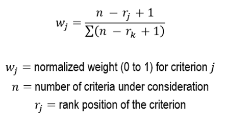
Ranking Methods

• Simplest method of all weighting techniques

• Every criterion under consideration is ranked in preference order

  • 1 is most important

• Once criteria are ranked, several procedures are available for generating numerical weights using the ranks

Rank Sum Equation

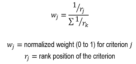
Rank Reciprocal Equation

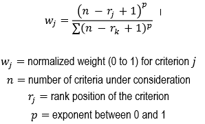
Rank Exponent Equation

• Like rank sum but you add an exponent

• Exponent = 0 would be equal weight across everything

• Exponent = 1 would be identical to rank sum

Ranking Methods Advantages and Disadvantages

• Advantages

  • Simple

  • Easy to implement

• Disadvantages

  • Limited to a small number of criteria

    • Larger the number of criteria, the more difficult it is to arrive at a reliable ranking since they would eventually lead toward tiny differences between weights

  • Lacks theoretical foundation

Point Allocation (Rating Method)

• Decision maker estimates weights on a predetermined scale (like 0-100)

• Each criterion would be allocated points with the sum of all points = 100 (0 means criterion can be ignored)

• Greater the points, greater the relative strength of the criterion

• Each criterion normalized using;

  • wj = rj / 100

Ratio Estimation (Rating Method)

• Assign 100 to the most important criterion

• Assign proportionally lower values to criteria of less importance

• Take ratio of each criterion to the least important criterion

• Ratio expresses relative desirability of a change from the worst level to the best level

• Normalized weights are derived at the end by dividing each ratio by the total of all ratios

Rating Methods Advantages and Disadvantages

• Advantages

  • Easy to understand, conceptualize as prioritizing where to put your money

• Disadvantages

  • Limited to small number of criteria

    • Same problem as ranking approaches

  • Lacks theoretical foundation

Calculation of Weighted Scores

• Determined based on the weights that are chosen and the type of influence each criterion has

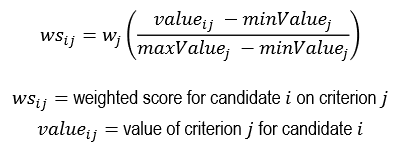
Positive influence weighted score

• How much more is a value compared to the min value in the range

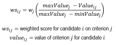
Inverse Influence Weighted Score

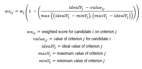
Ideal Influence Weighted Score

• How far is value from ideal

Trade Areas

• The geographical area containing (potential) customers served by a business or network of businesses

  • Can be scaled

    • Ex; applied to a community, business district, downtown

What would a trade area analysis tell you?

• Where a business’s customers are coming from

• How many potential customers live in a trade area

• Where to look for more customers

Who is concerned with trade area analysis?

• Retailers or commercial service providers

• Commercial property developers

• Real estate departments of retail chains

• Leasing companies

• Location analysts who work with any of the above

• Marketing firms who advertise for businesses

Factors that affect trade area size and shape

• Store size (attractiveness)

  • Area for furniture would be much larger than Starbucks

• Settlement patterns (residential density)

  • Dense area would mean more close

• Transportation network

• Barriers to movement

• Presence of competitors

Types of Trade Areas

• Convenience

• Destination

Convenience Trade Area

• Purchase of products and services needed on a regular basis

• Ease of access (travel time or distance)

  • Ex; groceries, gasoline, coffee, etc.