RSM483 Lecture 3 + 4

Home Price indices

• Tell us the price of the same good in different environments

• Here, we want to know the relative price of 1 unit of housing services

  • In different locations (spatial price index)

    • On average, what is the relative price of the same home located in Mississauga versus Toronto? (within metro region)

  • In the same location over time (more common)

    • On average, how much more is the same home in Canada worth in 2020 vs. 2010? (national)

Why is building home price indexes challenging

• Because homes are heterogeneous and the same home does not appear in different locations at the same time, nor does it stay the same over time, calculating home price indexes is challenging

spatial home price index

• Spatial: differences of the average home price across location. 

• Omitted location becomes baseline

• P is % difference in price of a typical home relative to baseline location. 

• Baseline becomes 100, and index reported as 100*e^p or 100(1+p)

Home Price Index

Difference in home prices over time. Challenge is that homes are different in unobserved ways and we often lack data on important home characteristics. to solve this, build a repeat sales index, which compares the sale price of the same home over time. 

Repeat Sales index

• Home price index built by measuring prices of same home over time. 

Labour supply and its 3 determinates

• Supply to each metro area is determined by wages, housing prices, and amenities

• Wages: more people want to live in a city if its wage is higher holding amenities and housing prices constant (labor supply curve slopes up) – Movement along curve

• Amenities: more people want to live in a city if it has better amenities, holding wages and housing prices constant (shifter of labor supply curve)

  • Make living in a certain area more attractive

• Housing prices: fewer people want to live in a city if its housing price is higher holding wages and amenities constant (shifter of labor supply curve)

  • If city is more expensive, even at same wage level, many people will not want to live there → curve shifts back

What shifts the labour supply curve?

Amenities and housing prices

More amenities — shift out

Higher prices — shift in as people leave. 

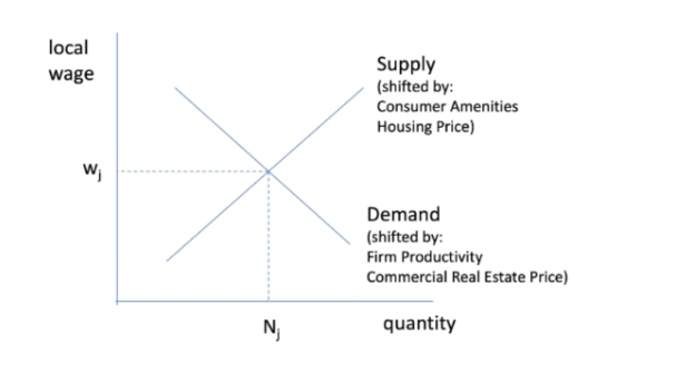
Labor demand 

determined by wages, firm productivity, and commercial real estate prices

• Wages: firms want to hire fewer people if city wage is higher holding productivity and real estate prices constant (labor demand curve slopes down)

  • Higher wages: hire less workers

• Productivity: firms want to hire more people if city productivity is higher holding wages and real estate prices constant (shifter of labor demand curve)

  • More productive: willing to hire more workers → shift curve out

• Real estate prices: firms want to hire fewer people if city real estate cost is higher holding wages and productivity constant (shifter of labor demand curve)

  • Need more office space for more workers → real estate expensive → hire less people → shift curve back. 

What shifts the labour demand curve?

firm productivity and commercial real estate prices

firm productivity up — hire more workers — demand curve shifts out

real estate prices up — expensive office space for each person — hire less people — demand curve shifts in

Housing supply curve

Real estate supply to each metro area is determined by price, construction costs and land availability 

• Housing/CRE price: developers willing to build more if real estate prices are higher holding other factors constant (floor space supply slopes up)

Other factors: if construction is more expensive or land is less available, developers will supply less housing at a given price (floor space supply shifter)

What shifts the housing supply curve?

if construction is more expensive or land is less available, developers will supply less housing at a given price (floor space supply shifter)

Housing demand curve

Real estate demand in each metro area is determined by price and the number of workers and residents in a metro area (workers = residents in this simple model)

• Price: people consume less housing & firms consume less CRE if prices are higher holding the number of workers and residents constant (real estate demand curve slopes down)

• Workers and residents: the more workers or residents, the higher is demand holding the price constant (demand curve shifters)

What shifts housing demand curve?

• # of Workers and residents: the more workers or residents, the higher is demand holding the price constant (demand curve shifters)

Compensating differentials in equilibrium

• Price differences compensate for quality differences in labor and product markets in equilibrium – This is a compensating differential

  • If two workers with the same skill make different wages at different jobs, the wage gap must reflect the difference in non-pecuniary benefits of the jobs

  • If not, the worker with the job that had the lower wage+benefit would move to the other job

Roback Model

• Consumers must have the same utility at all locations

  • Local amenity differences are compensated for by some combination of wage and cost of living (real estate price) differences across locations

  • Higher amenity places must have lower wages and /or higher cost of living

• Firms must have the same profit at all locations

  • Local productive amenity differences are compensated for by some combination of wage and cost of local input (real estate price) differences across locations

  • More productive places must have higher input costs

    • The same factors that affect consumer amenities can also influence firm productivity

Higher amenity places must have

• lower wages and /or higher cost of living

More productive places must have

• higher input costs

Consumers Perspective

says that amenities must make up the difference in income and housing prices s.t. Utility remain same for everyone.

Bid-rent

• The most a potential user would bid in rent for a plot of land

• Land goes to the highest bidder. 

• Arbitrage argument

  • If price > PV(rent) → demand for rental increases

  • If Price < PV(rent) → demand for ownership increases. 

Leftover Principle

• Leftover principal states that landowners get in rent what is left over in profits or consumer welfare after all other costs are paid

  • Assumptions

    • Firms profits are equal at all locations.

    • Consumer utility at all locations. 

• Basically firms are bidding up land price until they pay all their profits to get the land in equilibrium.

How is land a unique commodity?

• Land is a unique commodity because it has a fixed supply/quantity. 

• landowners will benefit if something happens that increases peoples WTP for their land

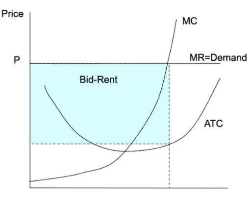
How does the bid-rent curve look in a graph?

all profits above atc below price where P = MC

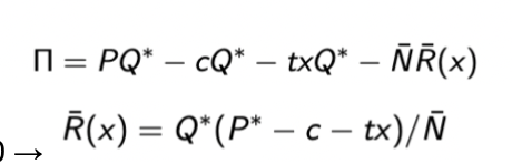
Leftover principle cost function

profit - revenue - costs - rent = 0 —> solve for rent. 

How does Bid-rend vary with location of property / distance from downtown. 

• As X increases, R(x) decreases as a compensating differential for higher transport costs.

• as transport cost becomes higher, curve becomes steeper

• as transport cost becomes lower, curve becomes flatter

• Slope = -t*q/N

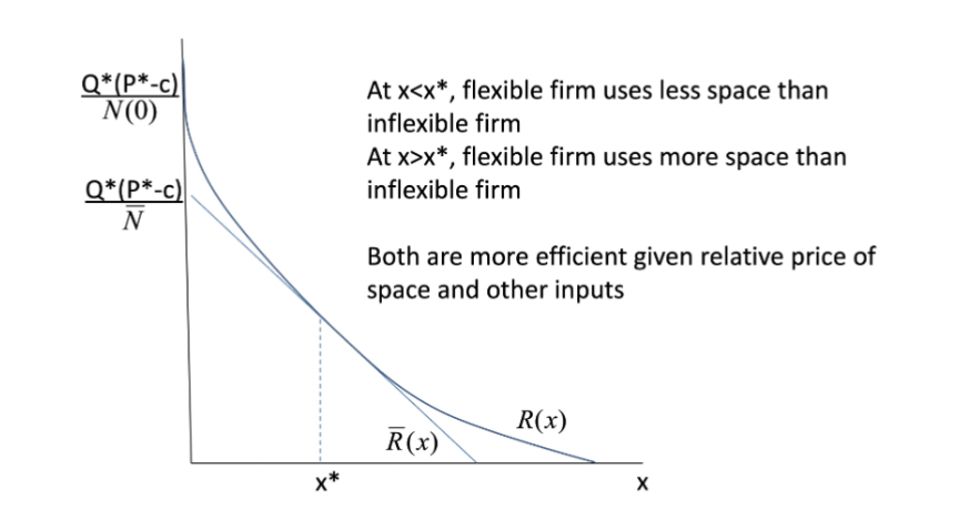
Adding ability to substitute land for capital

• Firms can now substitute away from land when it is more expensive.

• If firms has flexibility, firm can use less land and more capital and be more productive, thereby increasing profitability, thereby causing bid-rent to increase. 

Office firms and downtowns

firms enjoy higher productivity in denser environments

• > They pay higher wages and rents there than in other locations of the city

• > Productivity gains driven by agglomeration economies

• Because of productivity differences Those closer to DT are willing to bid more for spac

Households and bid-rent curves

• Household problem: choose z and s(x) to maximize utility subject to budget constraint

• Y - t*x = z + s(x) * R(x)

• solve for R(x) to get bid-rent curve.

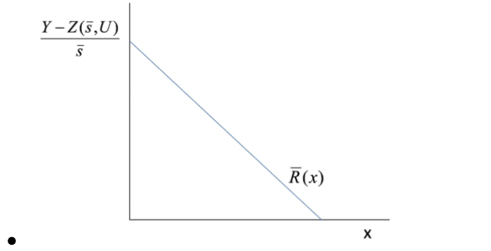
Fixed lot case

• If all homes have to be the same size

• Slope of the bid-rent is -t/s

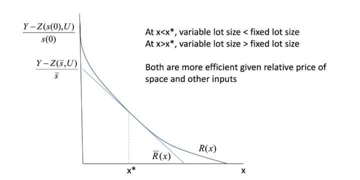
Variable lot case

• If house size is variable, they will substitute away from space when rent is high and towards it when rent is cheap. 

Open city and closed city

Open city model: Utility is fixed because people can freely move between cities until utility is equal everywhere. 

Closed city model: people cannot move out, so utility varies depending on the market conditions.