Computational Statistics

What is Landau (big O and little O) notation?

f(n) = O(g(n)) if

\lim_{n \to \infty} \frac{f(n)}{g(n)} \le C

for some C < \infty

Alternatively, this can be written as

f(n) = O(g(n)) if there exists a C < \infty and n_{o} such that for all n > n_0, f(n) \le Cg(n)

g(n) grows at least at the same rate asymptotically as f(n)

f(n) = o(g(n)) if

\lim_{n\to\infty}\frac{f(n)}{g(n)}=0

g(n) ‘dominates’ f(n)

Alternatively, this can be written as

f(n)=o(g(n)) if for all C < \infty, there exists an n_{o} such that for all n > n_0, f(n) \le Cg(n)

g(n) grows faster than f(n) asymptotically

We normally choose g to be as simple a function as we can and the slowest growing g that is possible, typically the next monomial

f(n) = 3n³ + 4n

f(n) = O(n³)

f(n) = o(n^4)

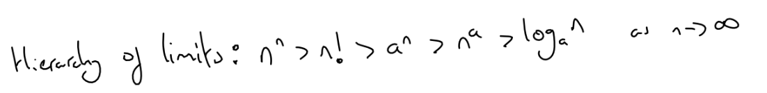
What is the hierarchy of limits?

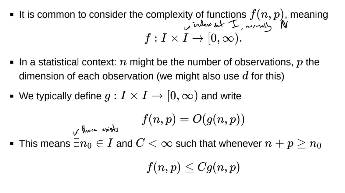
What is Landau notation for functions of multiple variables?

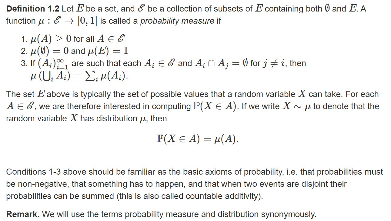
What is a probability distribution?

Sample space E, event space \mathcal{E}

\mathcal{E} cannot always be defined as all subsets of E, but throughout the course \mathcal{E} can be thought of as all subsets we are interested in

Often use the same symbol to denote a distribution and its density / mass function when there is no ambiguity, so

\pi(A) = \int_A \pi(x)dx

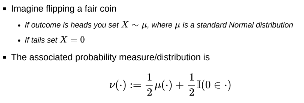
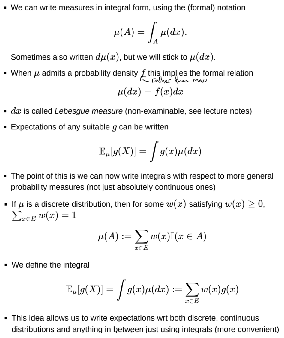
How can we represent random variables that are not fully discrete or continuous (i.e. mixed)?

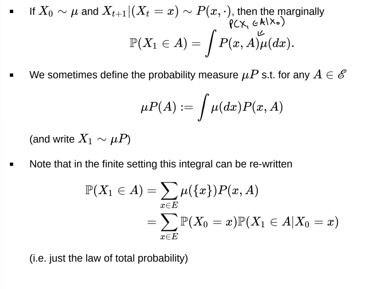
How can we write probability measures in integral form?

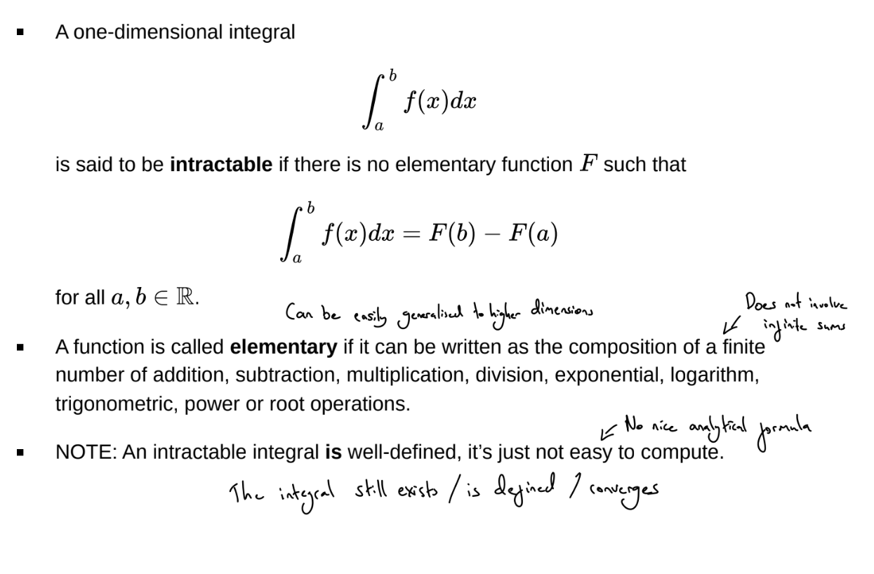
What is an intractable integral?

We may also have a tractable but expensive integral or sum: we call this computationally intractable

What is the trade off between analytical and numerical methods for calculating integrals?

With an analytical approach, we can achieve a closed form solution which is valid for all values of \theta. We can easily study how the integral changes with \theta, take derivations, etc.

With a numerical approach, we have a ‘black box’ procedure for computing the integral, which must be repeated for each different value of \theta. It’s therefore difficult to study how the integral changes with \theta. However, the numerical approach may be the only possible approach, or just faster and less computationally expensive

What are quadrature rules?

Numerical grid-based methods for approximating an integral as a weighted sum of values of the function at particular point in the interval, e.g. the trapezium rule

If N grid squares are needed to well approximate an integral in one dimension, then N^d = e^{dlog(N)} grid squares are needed in d-dimensions, so the complexity is exponential with dimension - curse of dimensionality

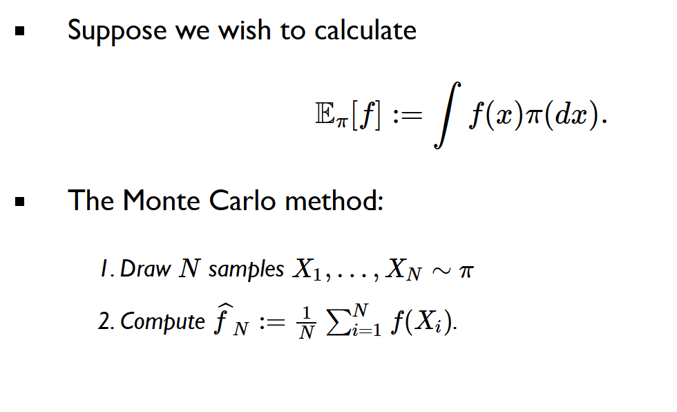
What is the Monte Carlo method?

This approach is identical in d-dimensions - so this approach can break the curse of dimensionality.

N typically does not need to grow with dimensions, but sampling may (or may not) become more difficult as N increases

Monte Carlo works because of the Law of Large Numbers and the Central Limit Theorem, which mean that for large N \frac{1}{N} \sum^N_{i=1}f(Xi) \approx \int f(x)\mu(dx)

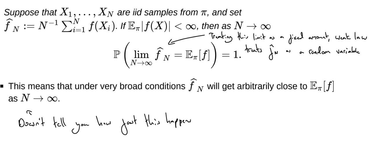
What is the strong law of large numbers?

What is the central limit theorem?

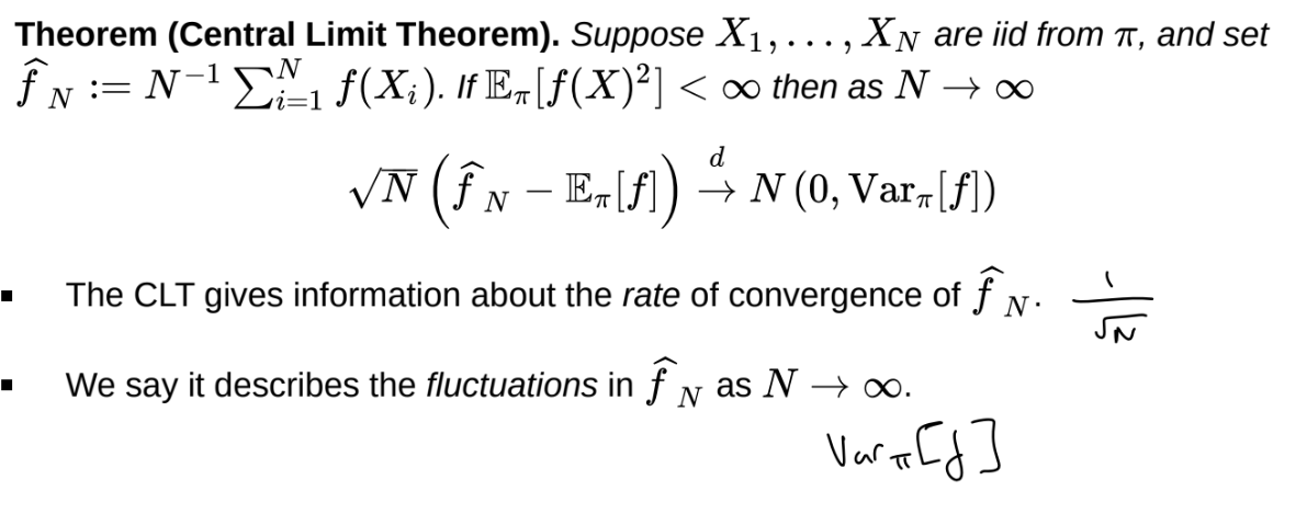
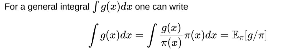
How can we use Monte Carlo to compute an integral that isn’t an expectation?

Need \pi to have at least as heavy tails as g

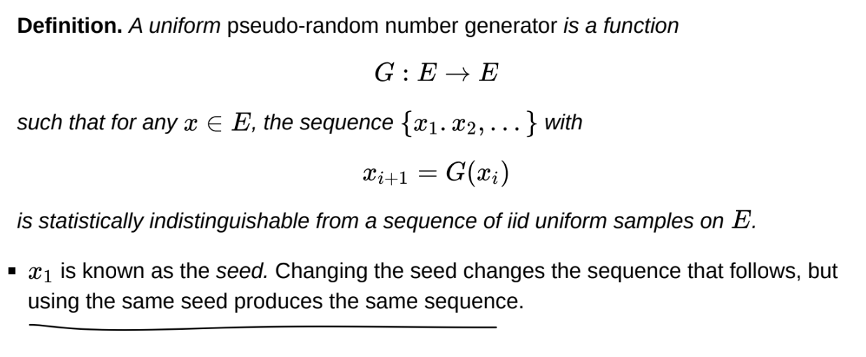
What is a PRNG?

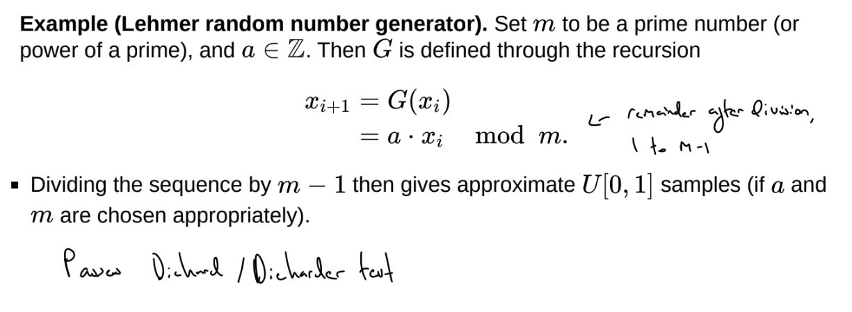
What is the Lehmer random number generator?

Any sample will be rational (some multiple of 1/(m-1)) and hence discrete

All samples from uniform distributions should be irrational - but values are an idealised approximation of irrational values

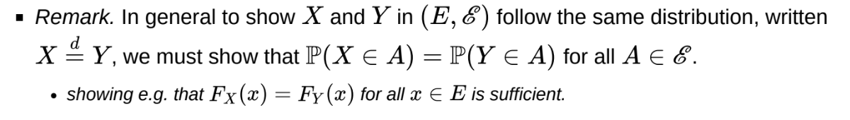
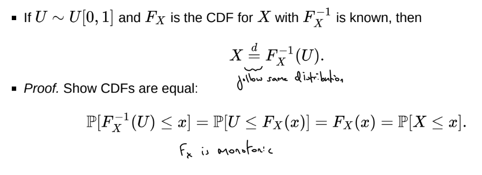
How can we show that X and Y follow the same distribution?

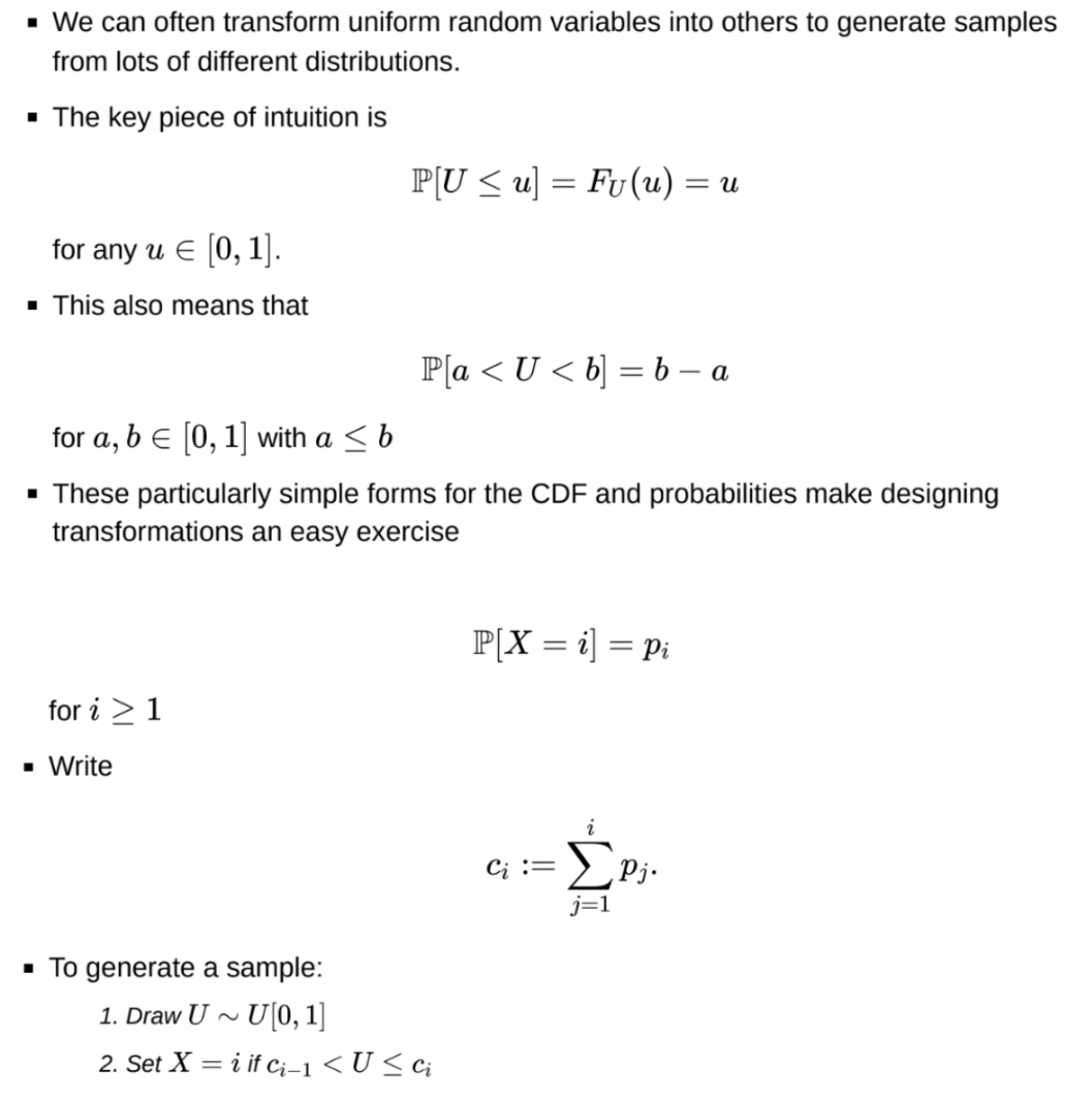
What is direct sampling?

Use the inverse CDF method for continuous cases - but this only works if F^{-1} is analytical

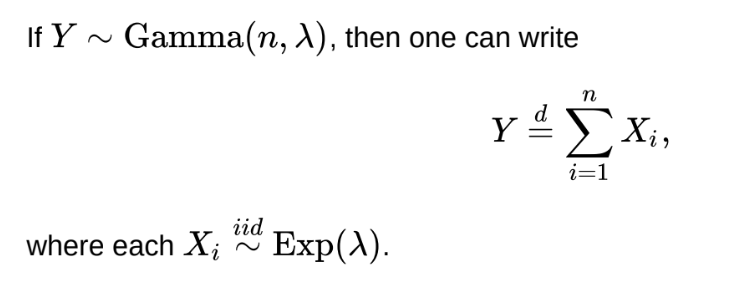
What is the relationship between Gamma and Exponential variables?

Can use to direct sample by using building blocks

What is the relationship between Chi-squared and normal variables

The sum of n standard normal variables follows a \mathcal{\chi}^{2}_{n} distribution

Can use to direct sample by using building blocks

What is the inverse CDF method?

What is indirect sampling?

What is rejection sampling?

The rejection sampling algorithm is:

set i ← 0

While i < N

• Draw X ~ q

• Draw U ~ U[0,1]

• If U\le\overline{}\frac{\pi\left(X\right)}{Mq\left(X\right)} , then accept X as a sample and set i ← i + 1

Set M= sup_{x} \frac{\pi(x)}{q(x)} (so that the ratio is always less than or equal to 1)

P[accepted]=\int q(x)\frac{\pi(x)}{Mq(x)}dx=\frac{1}{M}\int\pi(x)dx=\frac{1}{M}

So it is desirable to choose q s.t. M is as small as possible

The goal to make M as small as possible is achieved by setting q \approx \pi

In high dimensional settings this can be very challenging

For M to even be finite, meaning the algorithm is implementable, then the tails of density q(x)must be at least as heavy as those of \pi(x)

M (or some upper bound for it) must also be explicitly calculated

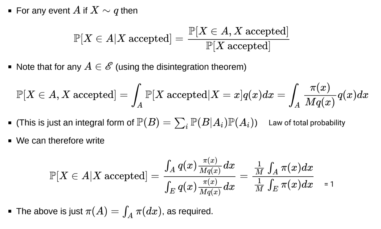
What is the proof that the rejection sampling algorithm produces samples from \pi?

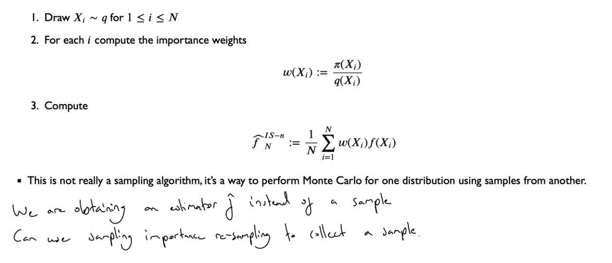
What is naive importance sampling?

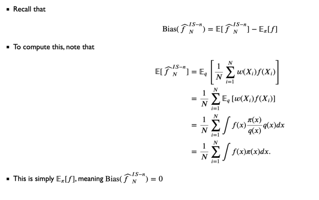
What is the bias of the naive IS estimator?

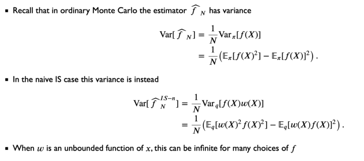
What is the variance of the naive IS estimator?

If \pi(X) is heavier-tailed than q(x), then w will be unbounded and variance will be infinite

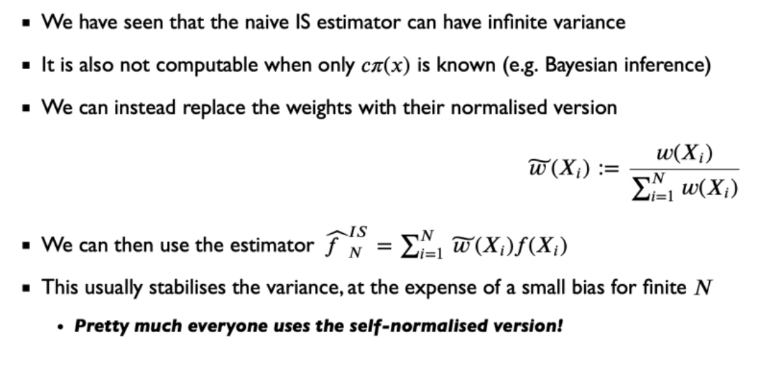
What is self-normalised importance sampling

where w(x_i) = \frac{\pi(x_i)}{q(X_i}

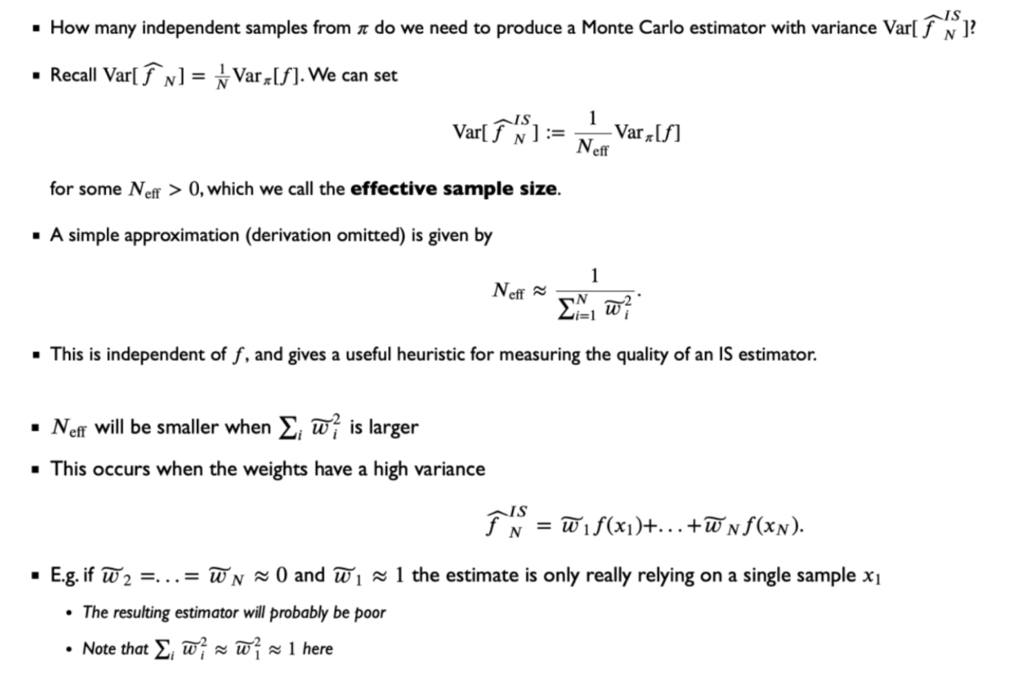
What is the effective sample size of the self-normalised importance sampling estimator?

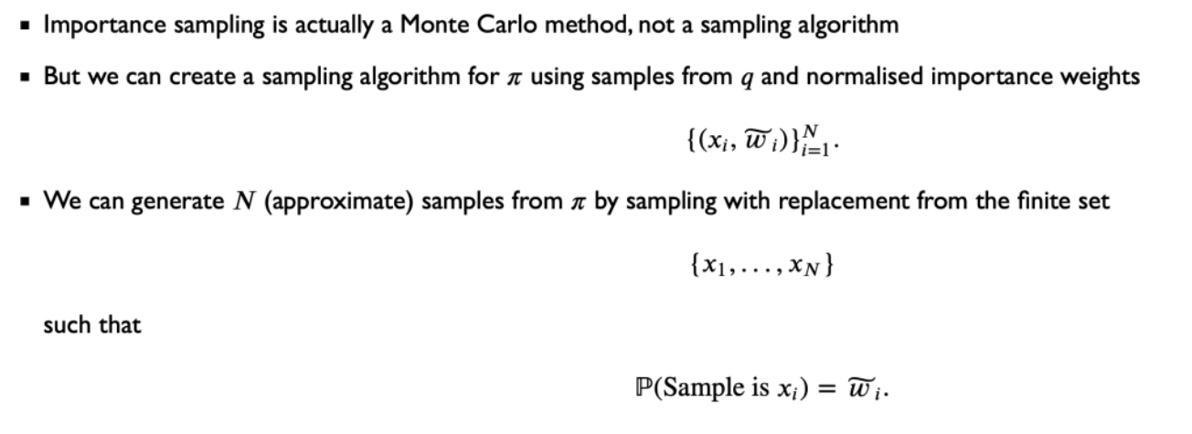
What is sampling importance resampling? (SIR)

The quality of this method is strongly linked to the quality / effective size of the importance sampling estimator. If \tilde{w_1} \approx 1, then every re-sampled point is likely to be x_1.

We can draw as many re-samples as we like, but they would only ever be a subset of the original sample, and we would likely have repeats

What are the pros and cons of rejection sampling vs importance sampling?

In importance sampling an upper bound on \frac{\pi(x)}{q(x)} is not needed, whereas in rejection sampling it is: otherwise M is undefined

In importance sampling, all samples are used, there is no ‘throwing away of samples’

However, unequal weights lead to a higher variance of the estimator. We want to maximise effective sample size, and so minimise \sum^N_{i=1} \tilde{w_i}²

We therefore still want to choose q to closely mimic \pi, and heavier tails in q are preferred

Given a sample from q of size n, in SIR, we can draw as many re-samples as we like, but they would only ever be a subset of the original sample and we would likely have repeats. In rejection sampling, we retain the accepted samples. The sample size is therefore random, but the sample will not contain repeated draws if the candidate distribution is continuous.

What is the permutation test?

H_0: \mu_X = \mu_Y

Where T is a test statistic, e.g. T=\left\vert\overline{x}-\overline{y}\right\vert{} where \bar{x} is the average of values with \gamma = 1 and \bar{y} is the average of values with \gamma = 0

The permutation test p-value is exact, rather than being based on asymptotic approximation.

The number of permutations grows factorially with both n and m - a huge computational barrier

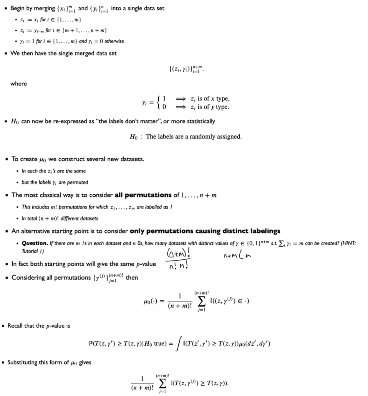
What is Monte Carlo permutation testing?

Rather than compute all (n + m)! permutations, simply compute a random subset

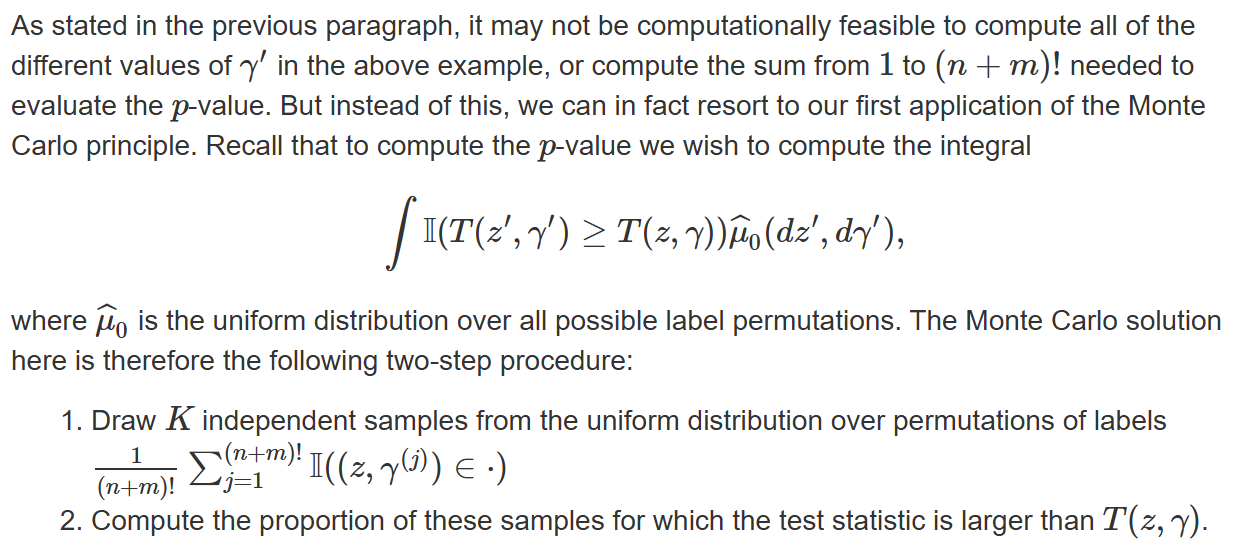
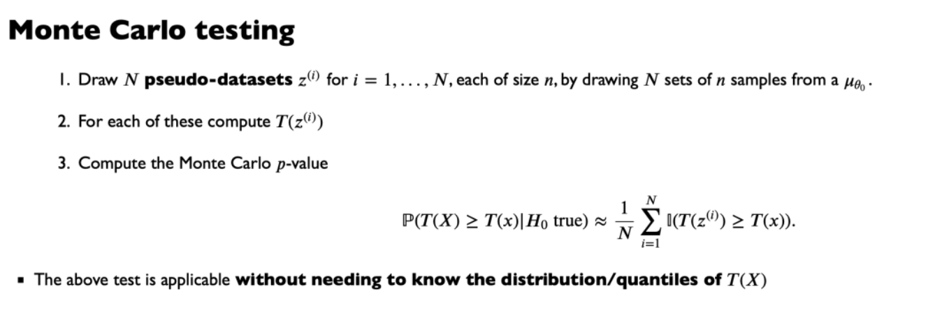
What is Monte Carlo testing?

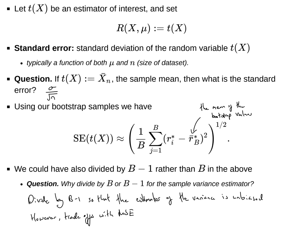
What is the Bootstrap?

We are trying to approximate the distribution of a random variable R(X, \mu) (the root).

We replace \mu with some \hat{\mu} based on the observations x, either using the empirical distribution or a parametric distribution.

We then draw B bootstrap samples (x_1^{*(j)}, …, x_n^{*(j)}) for j \in \{1, …, B\}, where each x_i^{*(j)} is a realisation of the random variable X_i^{*(j)} \sim \hat{\mu}

and compute r^*_j = R(x^{*(j)}, \hat{\mu}) for each j

The set \{r_1^*, …, r_B^*\} are then approximate samples from the distribution of R(X, \mu), and can be used to compute standard errors, construct confidence intervals and perform hypothesis testing. The quality of the approximation is determined by how well \hat{\mu} approximates \mu

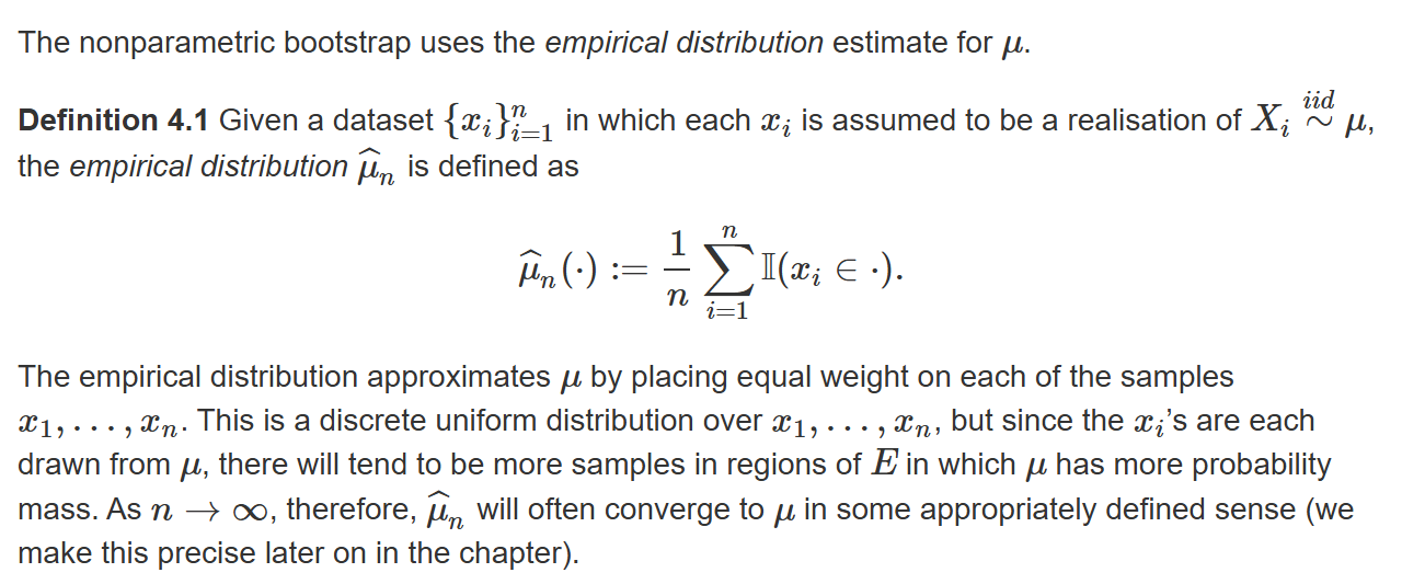
What is the nonparametric bootstrap?

The estimate \hat{\mu_n} is nonparametric because it does not assume a form for the distribution \mu that depends on a finite number of parameters. Sampling from \hat{\mu} equates to re-sampling with replacement from the set of observations x.

Can also used other non-parametric estimators for \mu other than the empirical distribution. In the smoothed bootstrap, we fit a non parametric density to observations and then sample from that, preventing repeats.

What are bootstrap standard errors?

How can we obtain bootstrap confidence intervals?

Note: when constructing confidence intervals for \theta in U[\theta_0, \theta_1], can never obtain more extreme values than min_{i}(X_{i}) and max_{i}(X_{i}), confidence intervals will be too high or too low

What is the parametric bootstrap?

The parametric bootstrap assumes that \mu follows some parametric form and then uses Maximum Likelihood Estimators to estimate parameters.

e.g. assume that \mu is Gaussian, and use the sample mean and sample variance as parameters

Advantages: can draw samples that are not in the original set of observations. does not have repeats, which are unrealistic for continuous data.

Disadvantages: unless the right distribution is chosen, asymptotic accuracy is sacrificed

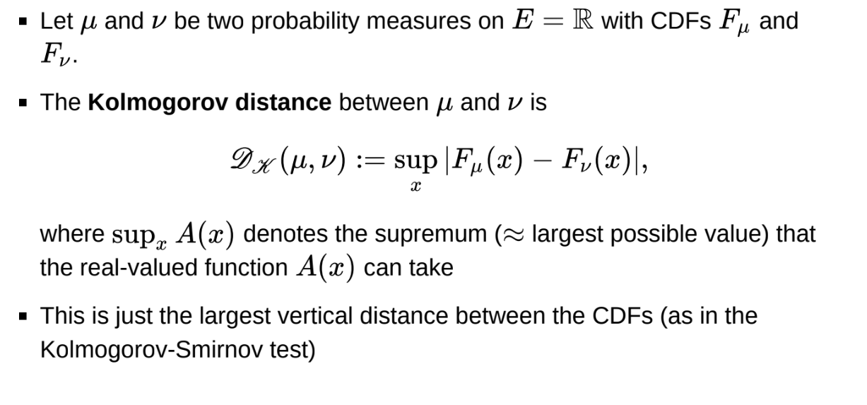
What is the Kolmogorov distance between probability measures?

Should we use the bootstrap?

Let the Kolmogorov distance D_{K}(\mu,\nu):=sup_{x}|F_{\mu}(x)-F_{\nu}(x)|

Let the empirical distribution \hat{\mu}_n(A) := \sum^n_{i=1} \textbf{1}(X_i \in A)

The Glivenko-Cantelli theorem finds that

lim_{n\to\infty}P(D_{k}(\hat{\mu}_n, \mu) = 0) = 1

Essentially, the bootstrap random variables are asymptotically valid whenever classical asymptotics are valid.

We can use the bootstrap in reasonable cases but this does not tell us that we can ever do better than using classical asymptotics.

For confidence intervals, the goal is to achieve the correct coverage:

P(L_\alpha(X) \le \theta \le U_\alpha(X)) = 1 - \alpha

Confidence intervals based on asymptotics typically have O(n^{-1/2}) error. Bootstrap percentile intervals also have O(n^{-1/2}) error but the constant is usually smaller.

Bias-corrected accelerated bootstrap intervals achieve O(n^{-1}) error, so achieve better coverage for moderate data sizes - bootstrap can beat asymptotics in the right setting

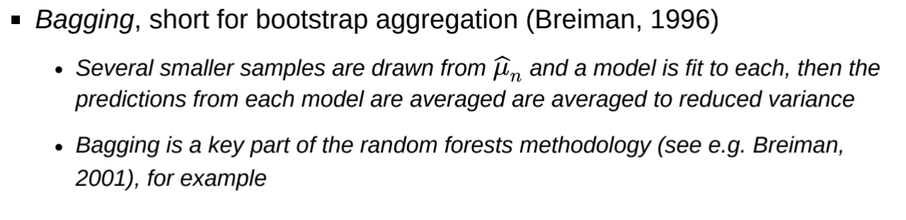
What is bagging?

Why can we not use direct sampling, rejection sampling or sampling importance re-sampling to sample from the posterior?

Direct sampling is usually not possible for complex models - e.g. need to find F^{-1}

Rejection and importance sampling usually suffer from the curse of dimensionality.

The probability of accepting candidate samples may decrease exponentially with dimension

The variance of weights in importance sampling typically grows exponentially with dimension, leading to a smaller effective sample size

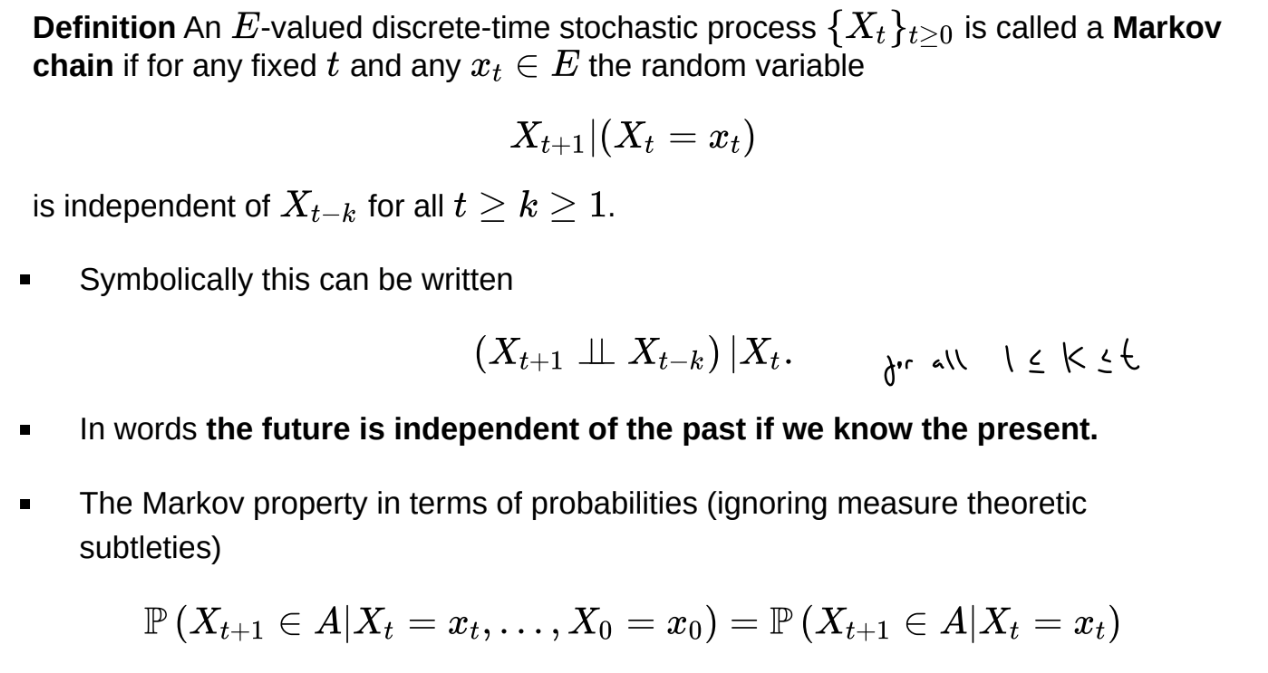
What is a Markov chain?

A Markov chain is a series of random variables \{X_t\}_{t \geq 0} (a discrete- time stochastic process) such that

(X_{t+1} \perp \perp X_{t-k}) | X_t

What is an E-valued discrete-time stochastic process?

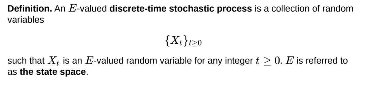
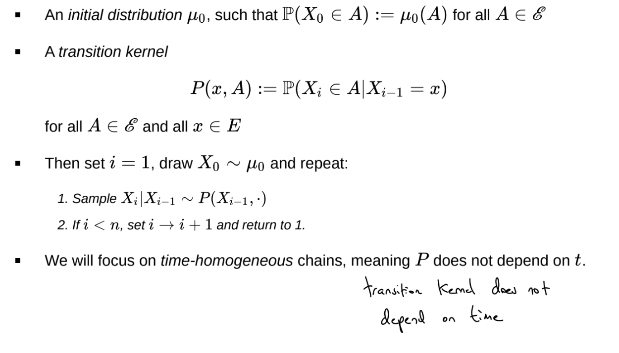
What do we need to simulate a Markov chain?

Can replace the transition kernel with a recursion, an equation showing how to turn X_i into X_{i+1}

X_{i+1} = f(X_i, \epsilon_{i+1})

where \epsilon_{i+1} is random noise

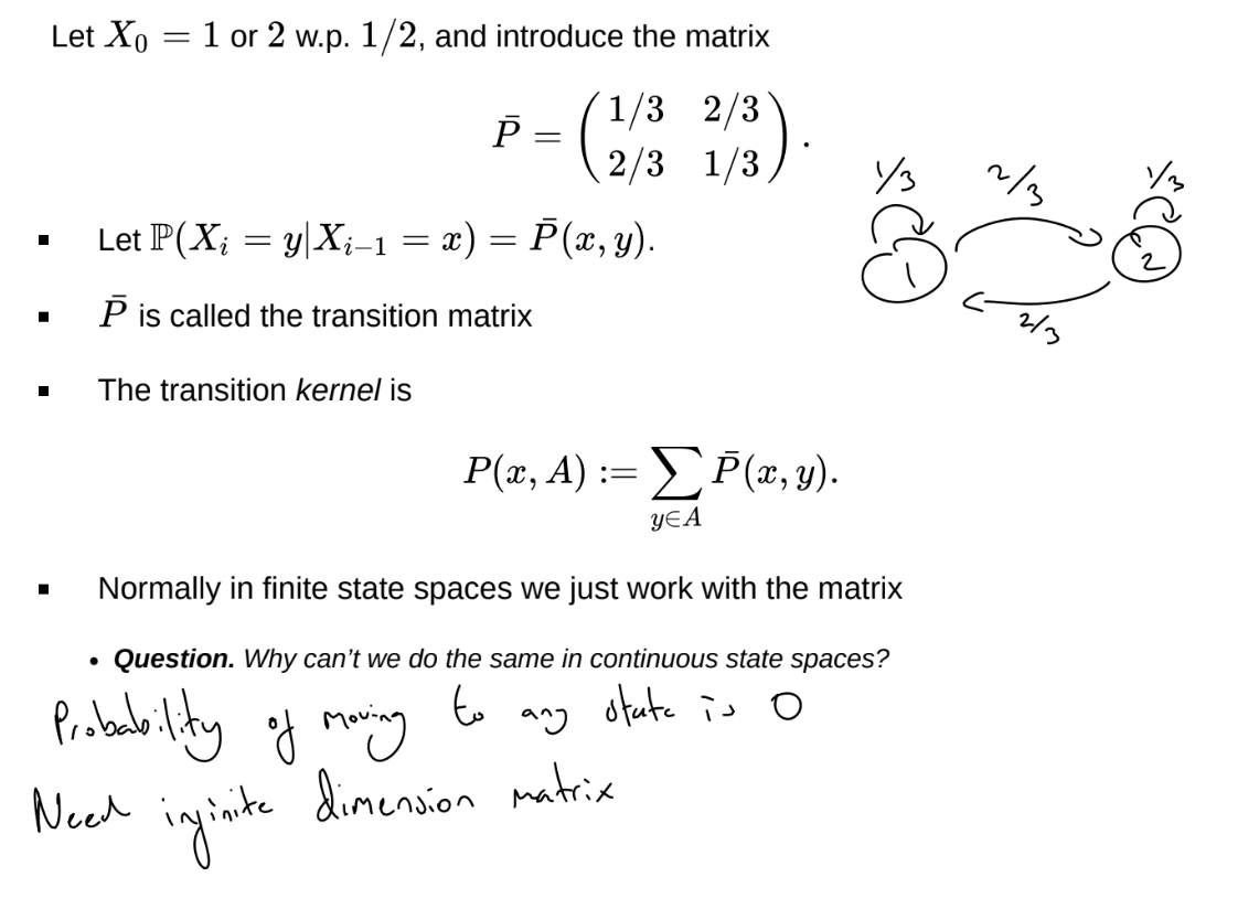
How can we characterise the transition kernel in a finite state space?

Note that

P(X_{t+n} = y | X_t = x) = \bar{P}^n(x,y)

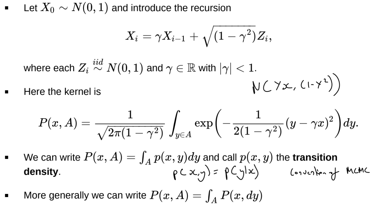
How can we characterise the transition kernel in a continuous state space?

What is the marginal distribution of samples in a Markov chain?

X_{n}\sim\mu P^{n}

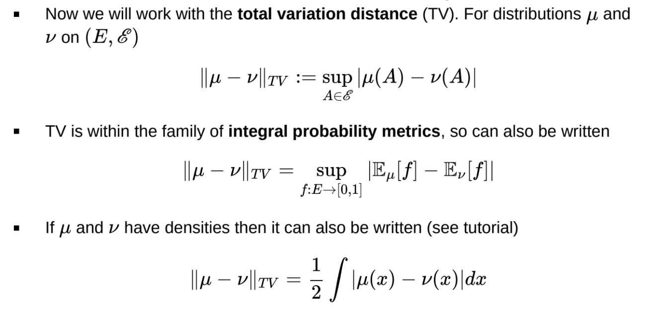
What is the total variation distance?

Supremum obtained in the set B := \{x \in E: \mu(x) > \nu(x)\} (and its complement)

What does it mean for a Markov chain to converge to equilibrium?

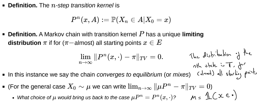
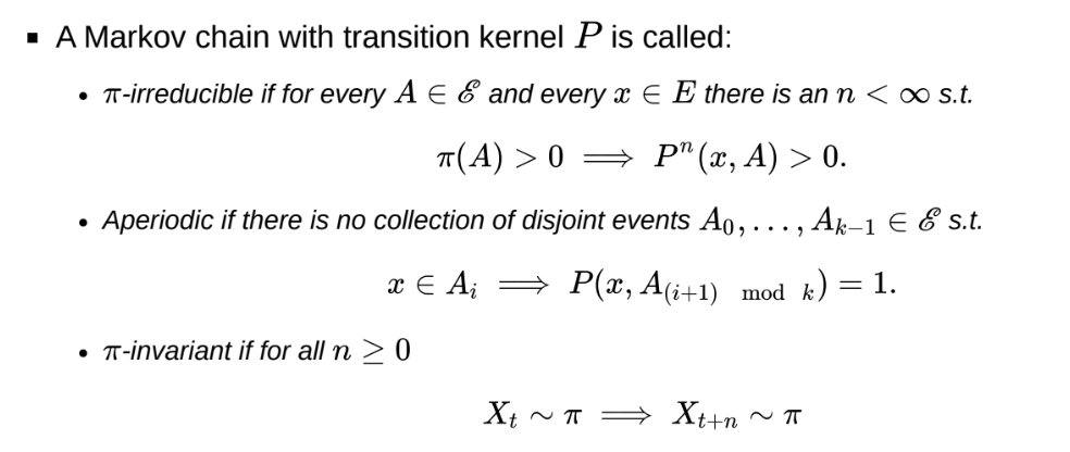
When do Markov chains converge?

If a Markov chain with transition kernel P is \pi-invariant, \pi-irreducible and aperiodic, then \pi is the unique limiting distribution for the chain

\pi-invariant: if the chain enters / starts in \pi, it stays in \pi

\pi-irreducible: the chain can reach any state with positive probability in \pi with positive probability, ensuring it does not get stuck in a subset of the state space.

aperiodic: if the chain is periodic, the chain will oscillate rather than converge. Can show the chain is aperiodic if there is a non-zero probability it remains at the same value.

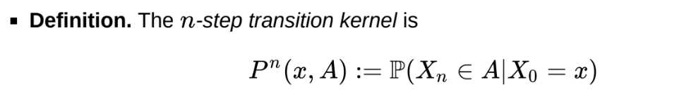
What is the n-step transition kernel?

If there is a transition matrix P, the n-step transition kernel is P^n(x, A)

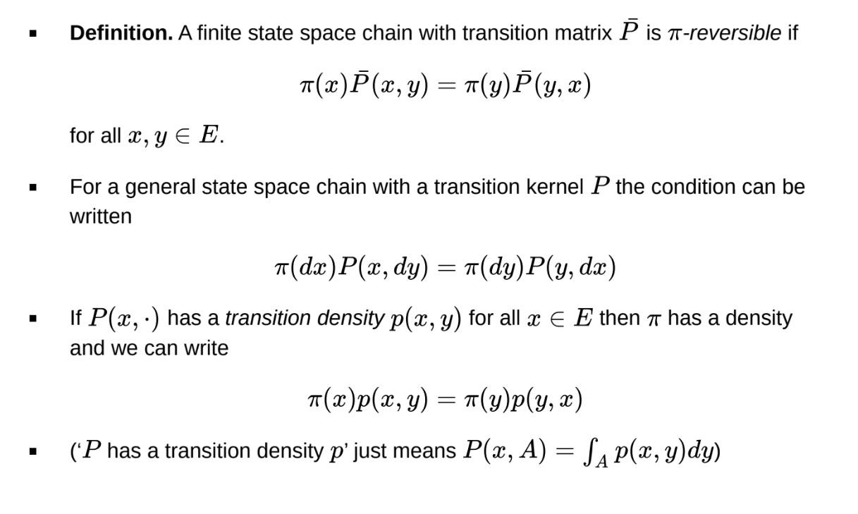
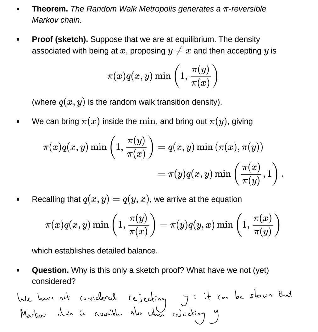
What is \pi-reversibility?

These are the “detailed balance equations”

If a Markov chain is \pi-reversible, then it is \pi-invariant.

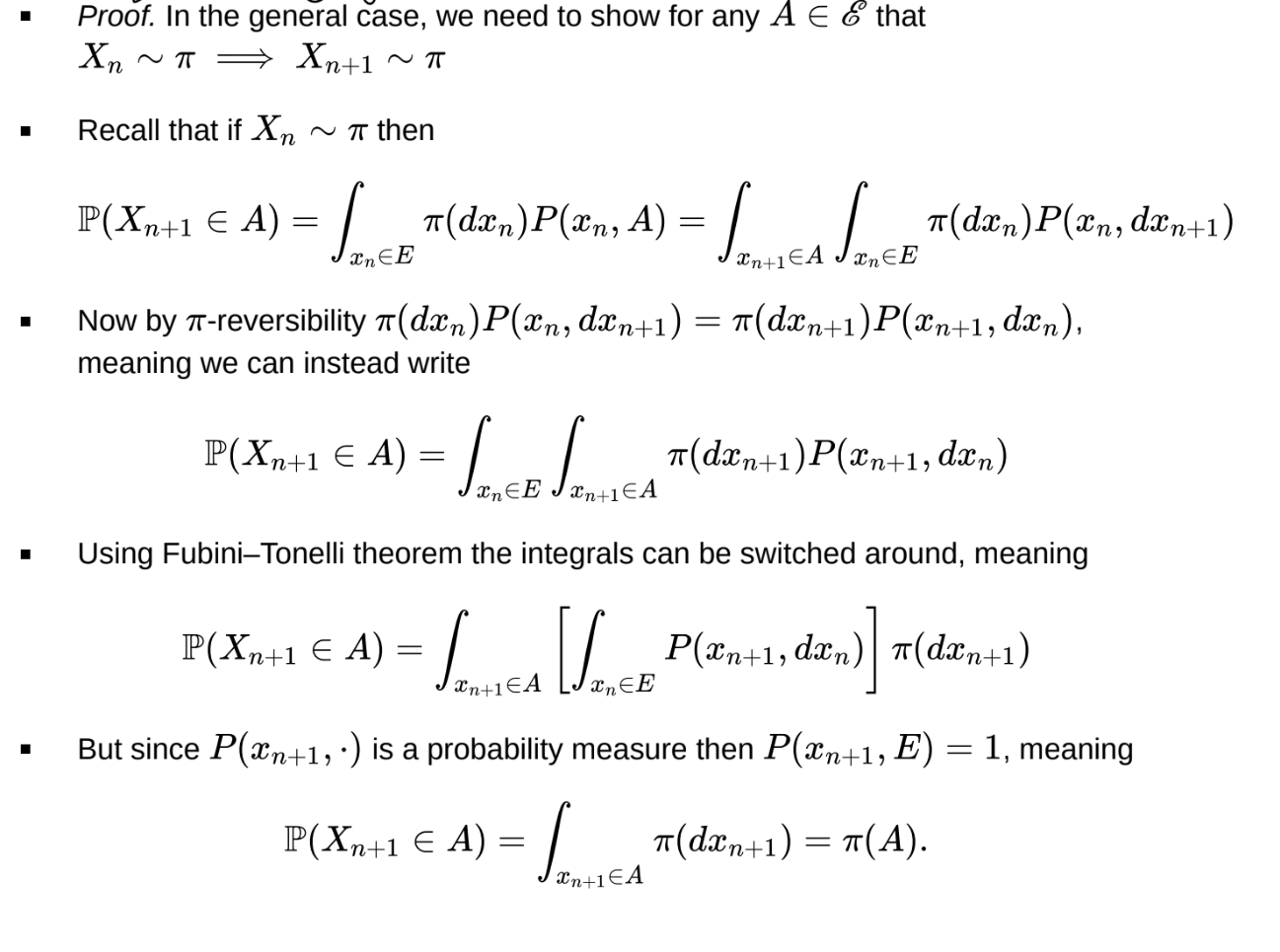
What is the proof that \pi-reversibility → \pi-invariance?

Markov chains can be \pi-invariant without being \pi-reversible

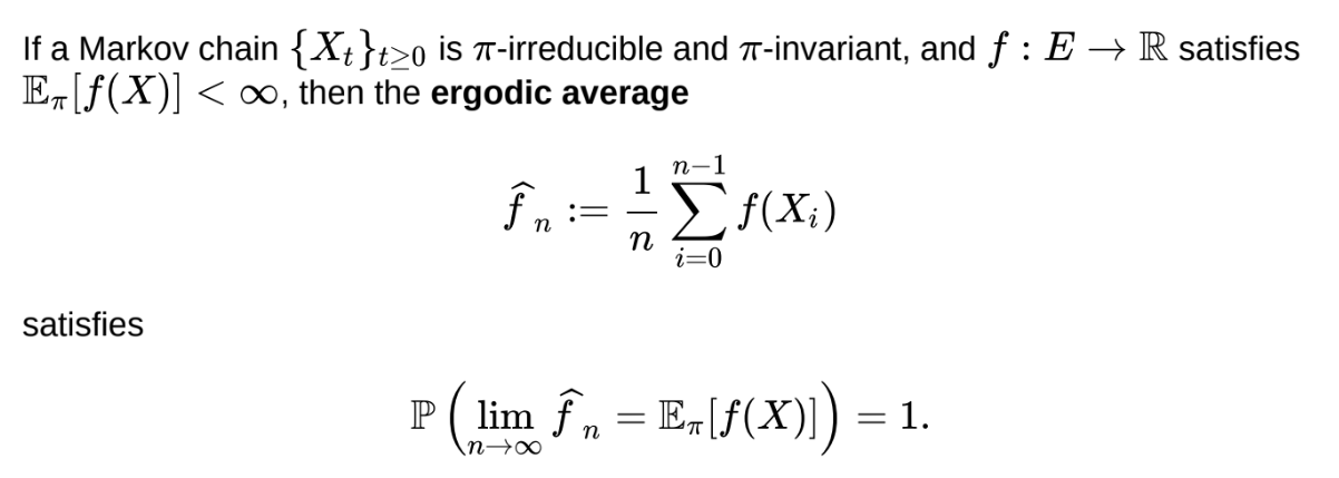
What is the Markov chain ergodic theorem?

Does not require aperiodicity

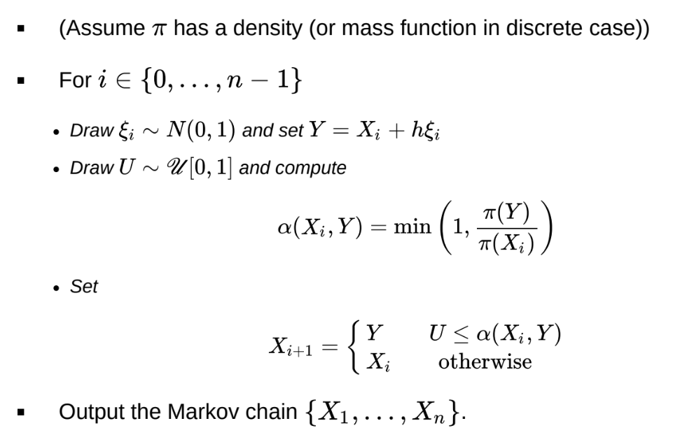
What is the random walk metropolis algorithm?

If \pi(Y) \geq \pi(X_i) \impliesAccept the move

Uphill moves are always accepted, downhill moves are sometimes rejected.

Therefore, the Markov chain spends more time in regions of higher probability under \pi

What is the sketch proof that the random walk Metropolis generates a \pi-reversible Markov chain?

What is the optimal h for the Random Walk Metropolis algorithm?

The step-size h is a tuning parameter that determines the acceptance rate. If h is too large, the acceptance rate will be very low and the chain will be ‘sticky’. If h is too small, the acceptance rate will be very high, and so the Markov chain will be close to a random walk. In both cases, there is significant autocorrelation between samples and the chain doesn’t explore the sample space quickly.

There is a sweet spot for h. In 1D, the optimal acceptance rate is typically around 44%. In the high dimensional settings, d \geq 5, it is around 23%

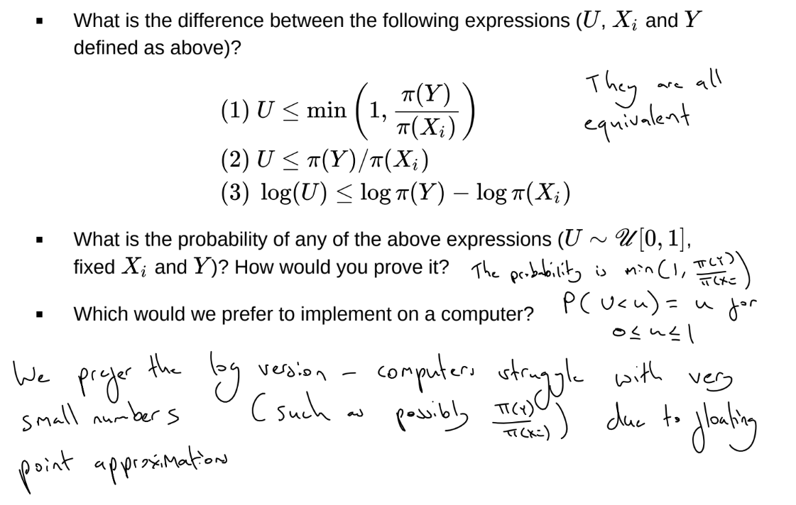
How do we carry out rejection for the Random Walk Metropolis algorithm on a computer?

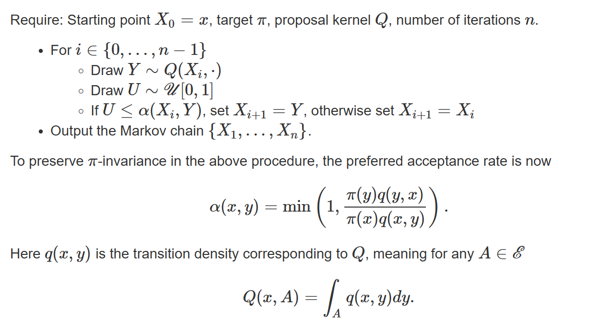
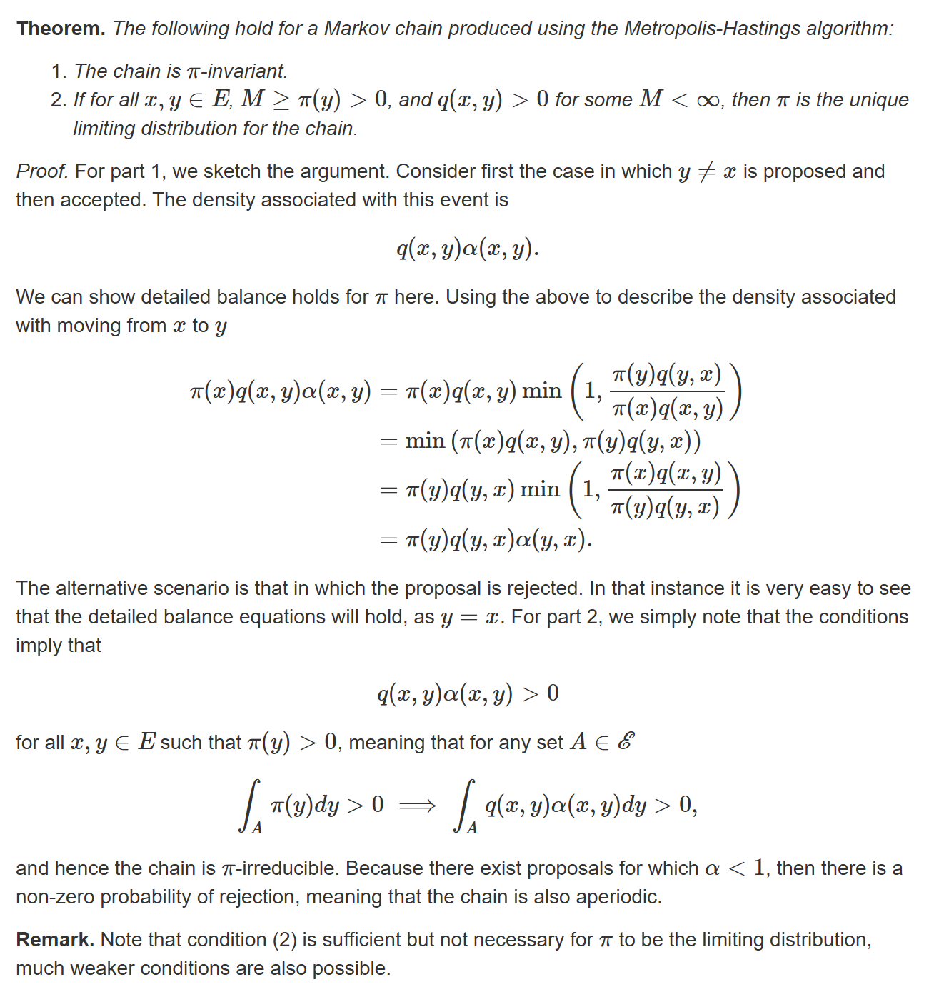
What is the Metropolis-Hastings algorithm?

What is the proof that a Markov chains produced using the Metropolis-Hastings algorithm is \pi-invariant and that \pi is the unique limiting distribution of the chain?

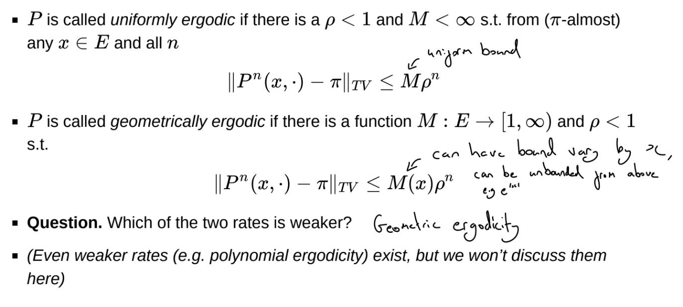
What are uniformly ergodic and geometrically ergodic transition kernels?

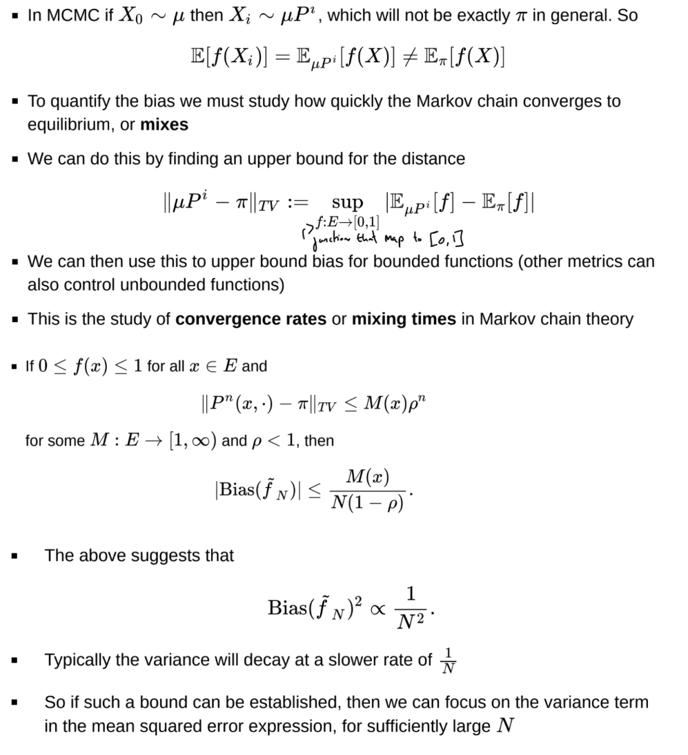
What is the bias of the MCMC estimator?

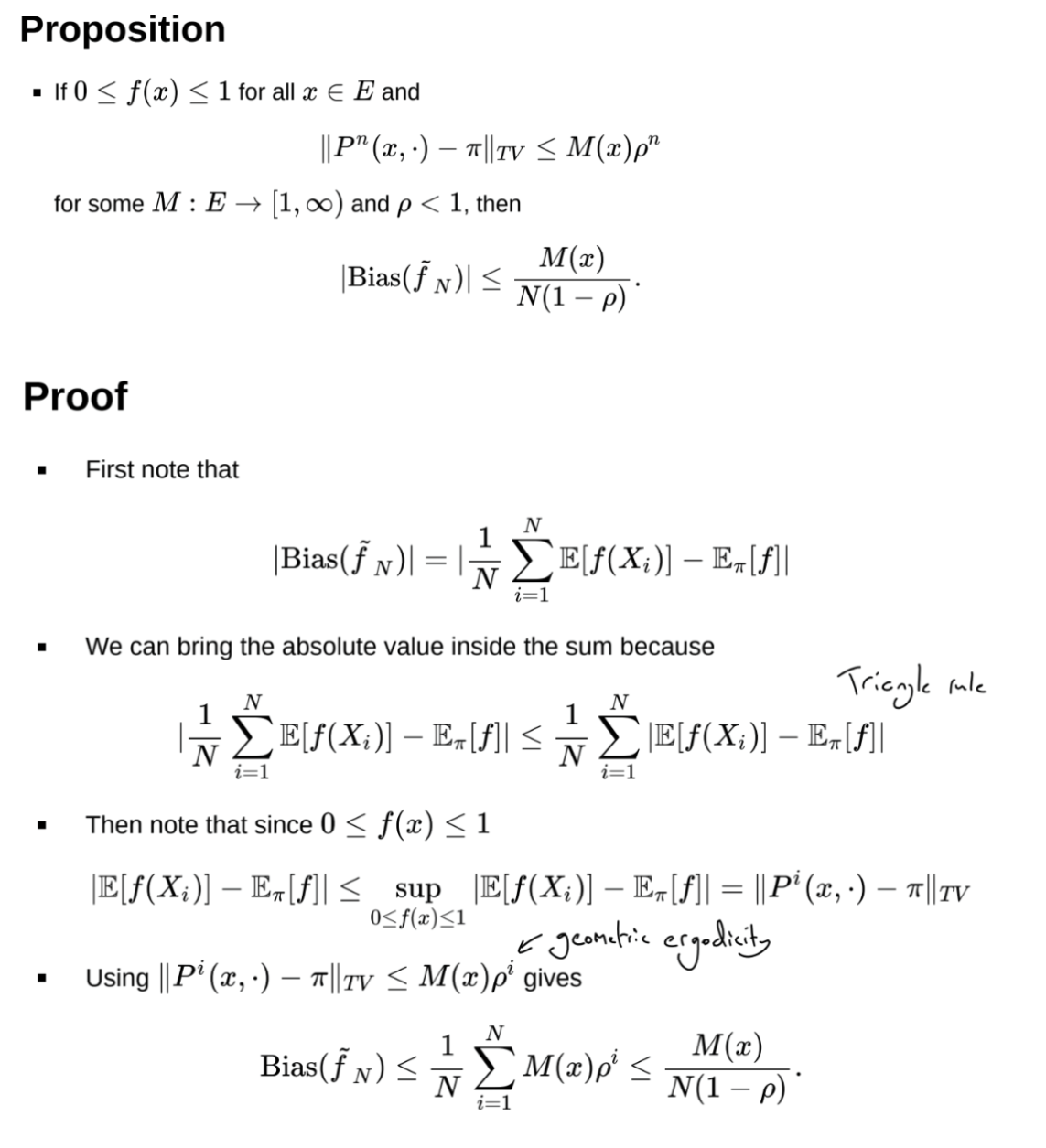
What is the proof of the upper bound of the bias of the MCMC estimator?

Assuming P is geometrically ergodic

When are Markov chains geometrically ergodic?

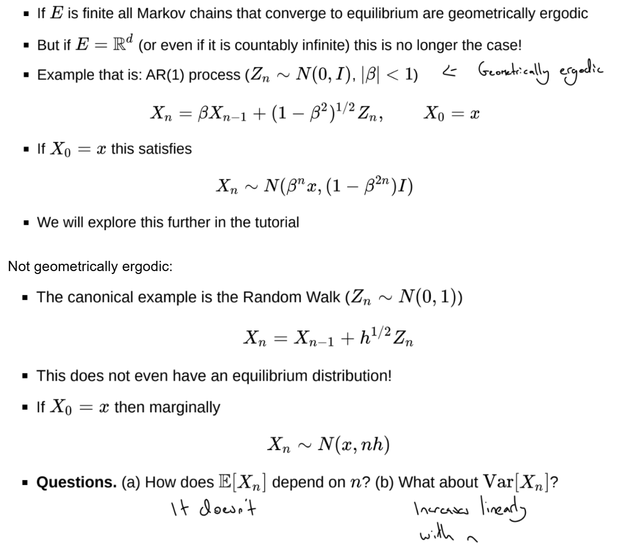
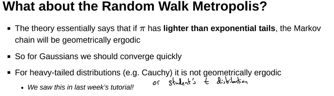
When is the random walk metropolis algorithm geometrically ergodic?

Cauchy acceptance rate is too high, similar to random walk

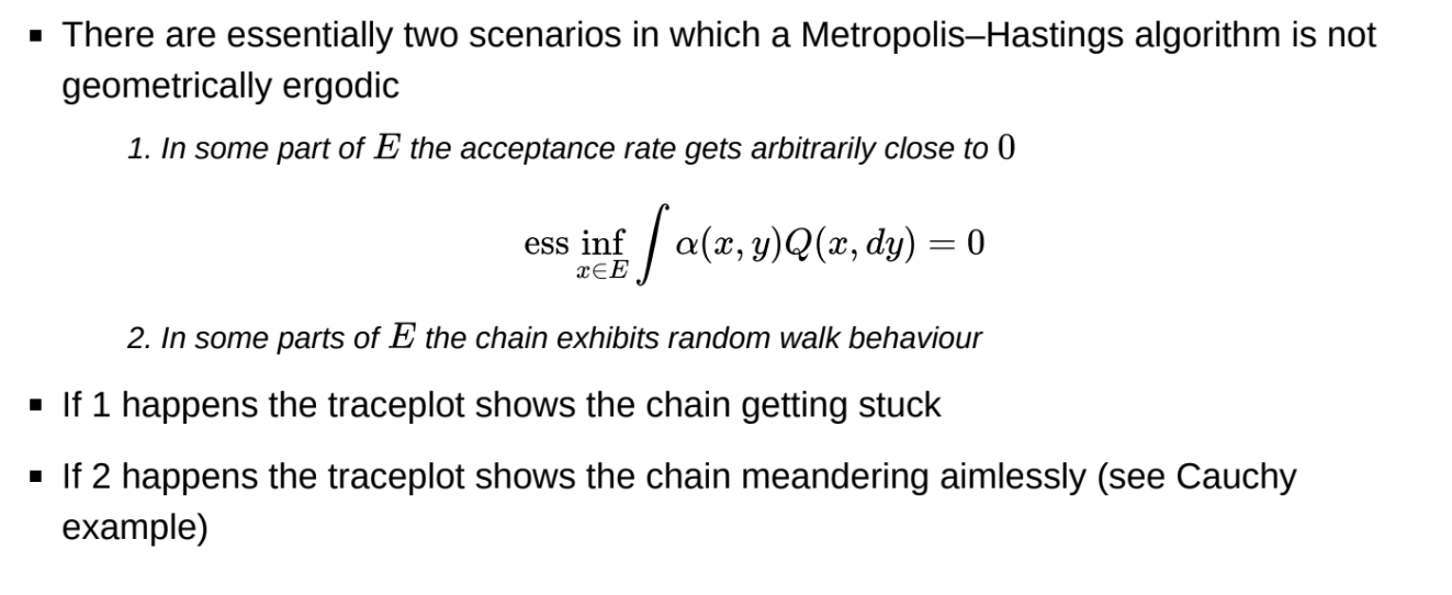
When is a Metropolis-Hastings algorithm not geometrically ergodic?

Ess inf: essential infimum / lower bound

In some part of E, the acceptance rate gets arbitrarily close to 0 or to 1. Chain gets stuck or exhibits random walk behaviour

1: acceptance rate too low

2: acceptance rate too high

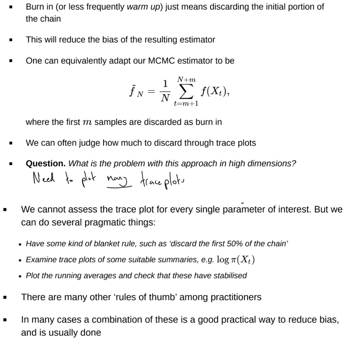
What is burn in?

Or use Gelman-Rubin diagnostic

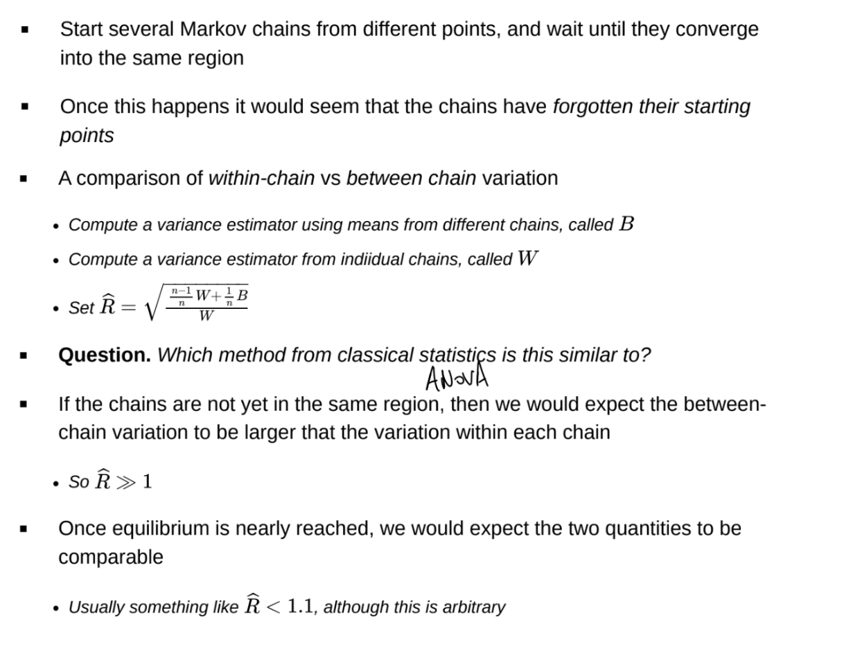
What is the Gelman-Rubin diagnostic?

Can be used to determine burn in

What is the variance and asymptotic variance of an MCMC estimator?

Under iid sampling from \pi, covariance of samples will be 0

We multiply Var[\tilde{f_N}] by N, as otherwise the asymptotic variance will tend to 0 and N tends to infinity.

Can have variance lower than usual MC estimator if covariance between Xs is 0 - antithetic sampling, samples spread out over the support of the distribution quickly

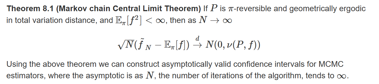
What is the Markov chain central limit theorem?

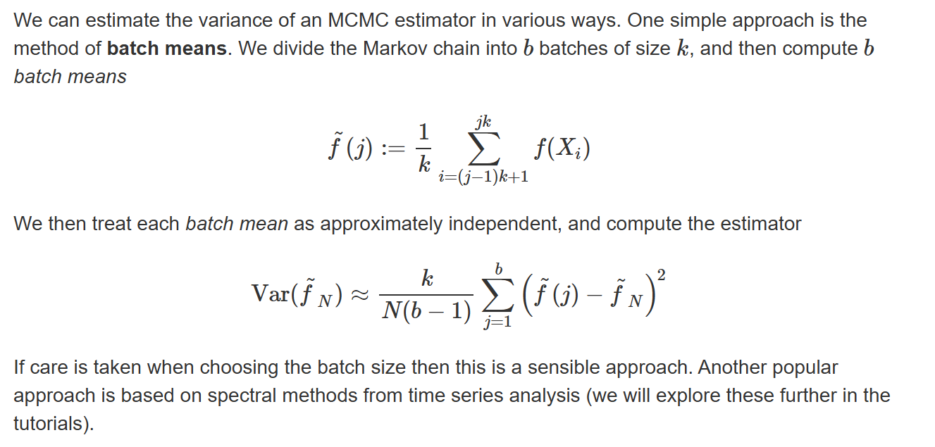
What is the method of batch means?

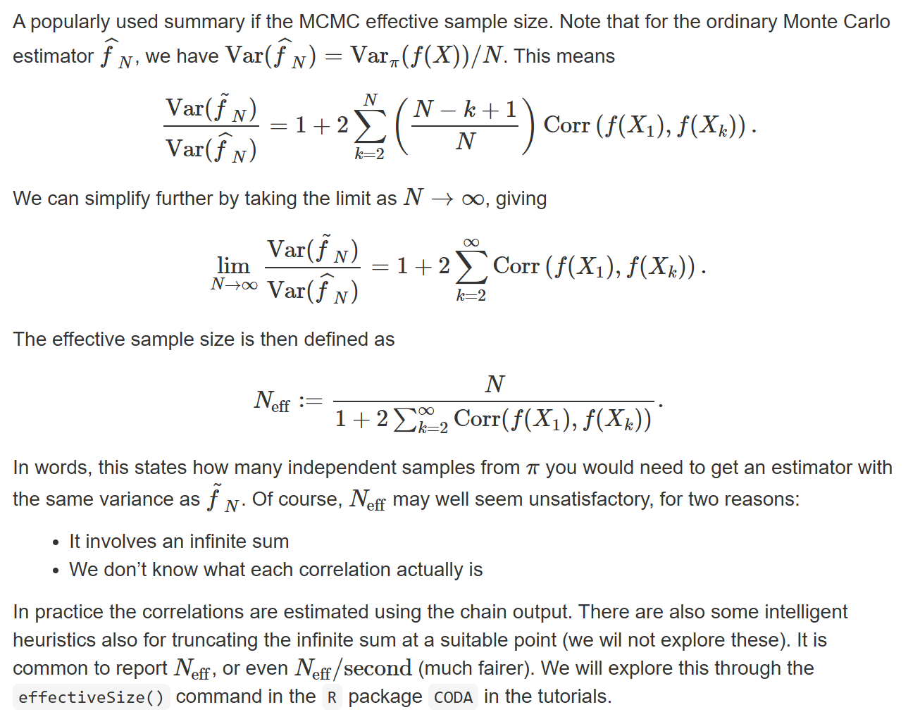
What is the MCMC effective sample size?

How do we measure computational complexity in MCMC?

There are many ways to measure computational complexity in MCMC

A popular strategy is cost per iteration \times converge rate / mixing time

Another is to only discuss the mixing time, since cost per iteration is more problem dependent

Both costs should be written as a function of dimension d. Generally we desire complexity to be polynomial, not exponential, in d.

The cost per iteration of a Metropolis-Hastings algorithm. This depends on the algorithm and the target distribution. There is the cost of the proposal and then the accept-reject decision. Generally, the most expensive part is calculating \pi(x) and \pi(y)

The converge rate / mixing times depend strongly on both the algorithm and \pi. If \pi is suitably nice, then mixing time of random walk Metropolis is O(d)