LEC 11: CH 15 ANOVA

Comparing the means of more than two groups

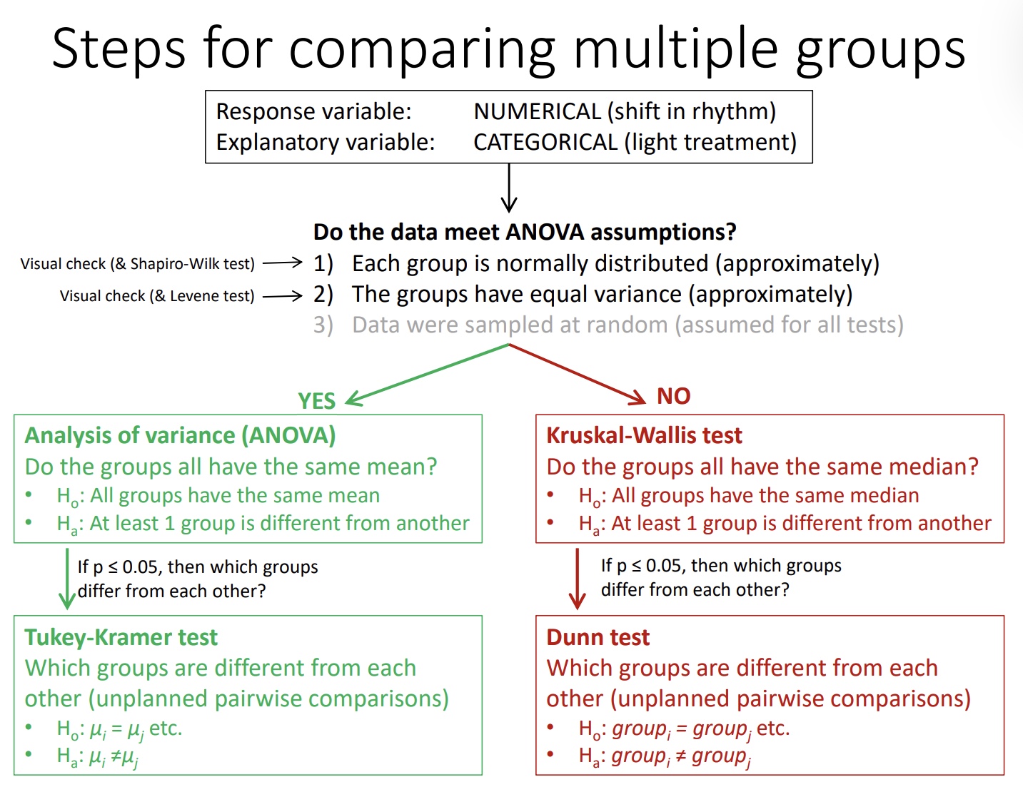
Steps for comparing multiple groups

Analysis of variance (ANOVA)

Similar concept to t-test: compares means of numerical variables for data grouped by a categorical variable (factor)

• However, it can compare two or more groups (unlike a t-test, which only compares 2 groups)

• It tests whether all the groups have the same mean (or not)

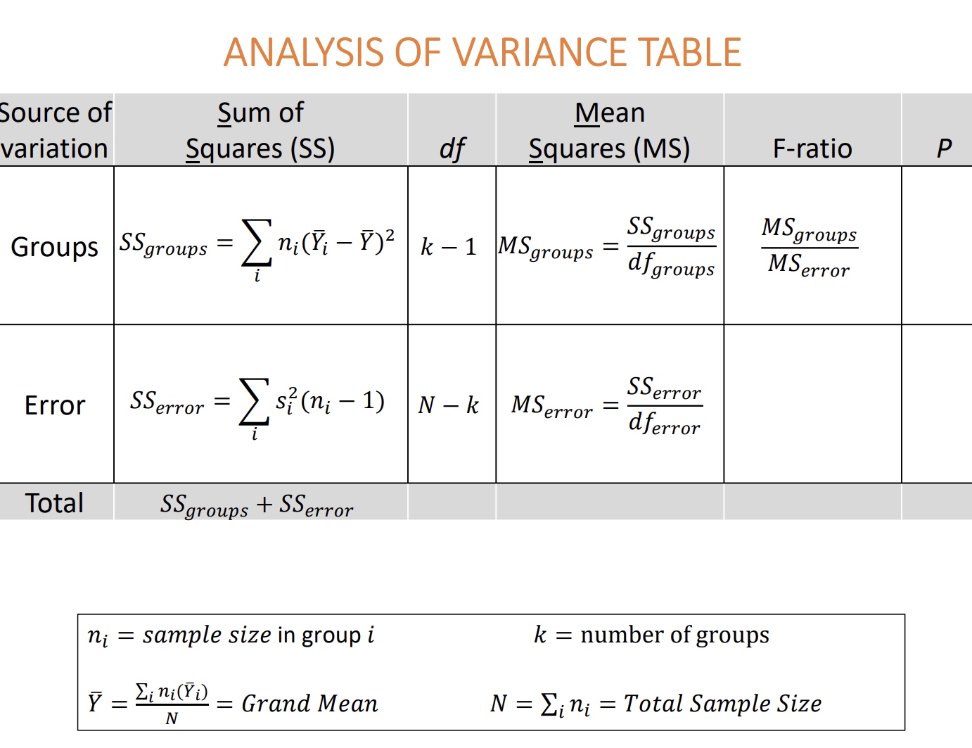
An ANOVA partitions the variance in the data

Total variation = variation among groups + variation within groups

how to interpret this chart

omponent	What It Means
Source of Variation	What’s causing the differences? Two sources: Groups and Error
Sum of Squares (SS)	Measures the variability: – SS<sub>groups</sub>: variation between group means – SS<sub>error</sub>: variation within each group
Degrees of Freedom (df)	Number of values free to vary: – df<sub>groups</sub> = k − 1 – df<sub>error</sub> = N − k
Mean Squares (MS)	Just the average variation: – MS = SS ÷ df
F-ratio	F = MS<sub>groups</sub> ÷ MS<sub>error</sub> It tells you whether between-group variability is much bigger than within-group variability
p-value (P)	Tells you if the F-ratio is large enough to be statistically significant (i.e., likely due to real differences rather than chance)

---

📐 How to Interpret Results

• If p < 0.05 → reject the null hypothesis:
  ✅ At least one group mean is significantly different.

• If p ≥ 0.05 → fail to reject the null:
  ❌ No evidence of a difference in means

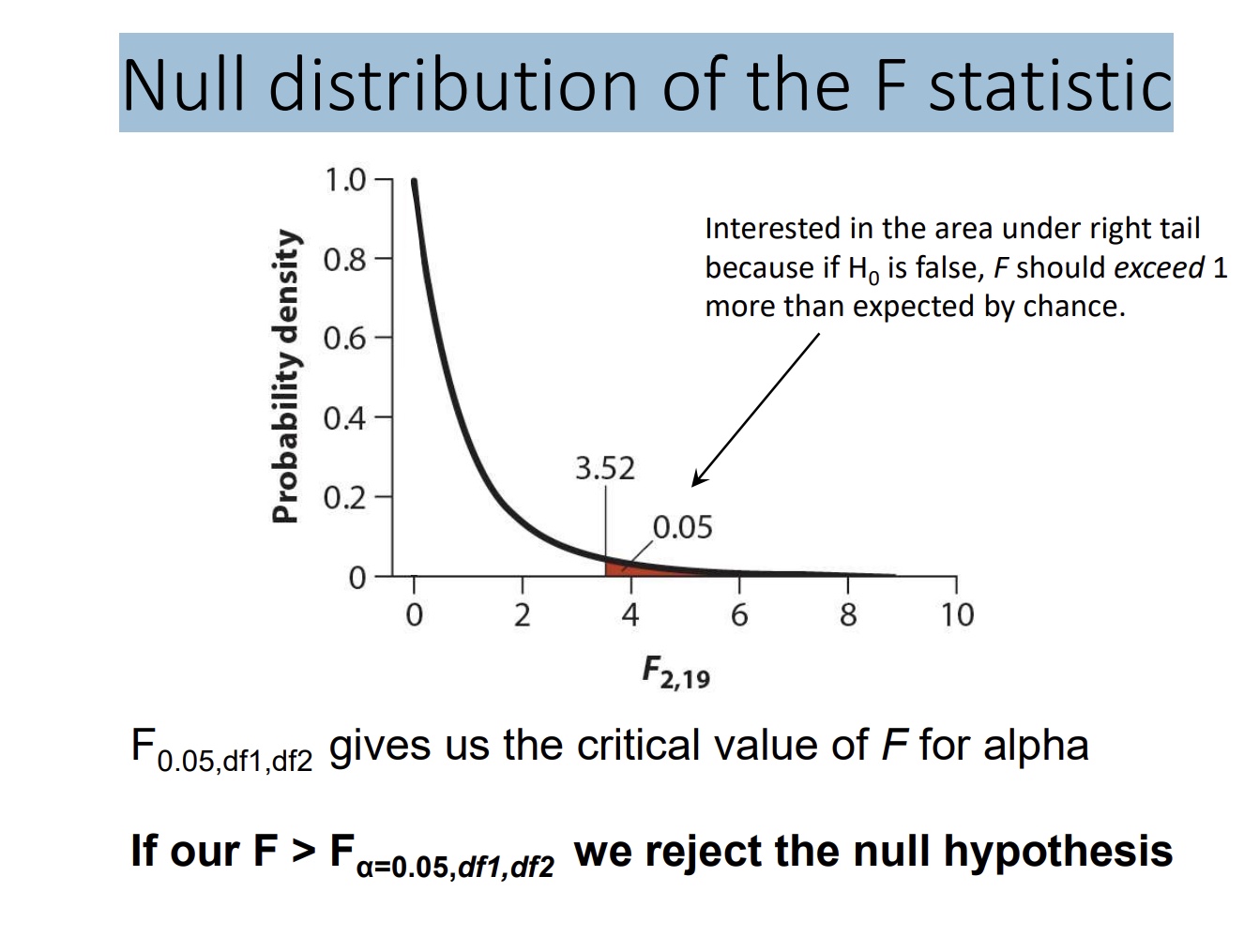
Null distribution of the F statistic

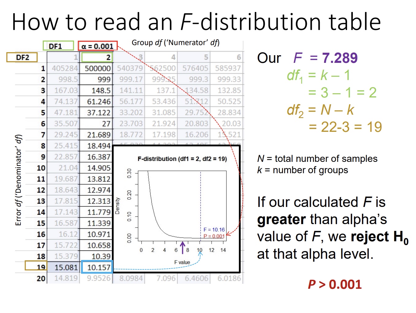
How to read an F-distribution table

📖 How to Read It Step-by-Step 1. Know Your Two Degrees of Freedom (df):

In ANOVA, you need:

• df₁ (numerator): between-groups degrees of freedom → usually k - 1

• df₂ (denominator): within-groups degrees of freedom → usually N - k

📝 Example: If you're comparing 3 groups (k = 3) with a total of 30 subjects (N = 30):

• df₁ = 3 - 1 = 2

• df₂ = 30 - 3 = 27

---

2. Decide on Your Significance Level (α):

Usually:

• α = 0.05 (most common)

• α = 0.01 (stricter)

You will use the column for your α-level.

---

3. Find Your Critical F-value in the Table:

• Go to the row for df₁ (numerator)

• Go across to the column for df₂ (denominator)

• Look under the correct α (usually a separate table or section)

✅ This value is your critical F-value

---

4. Compare Your Calculated F-statistic:

If...	Then...
F<sub>calculated</sub> > F<sub>critical</sub>	✅ Reject H₀ → Significant difference
F<sub>calculated</sub> < F<sub>critical</sub>	❌ Fail to reject H₀ → Not significan

Conclusion from the ANOVA

H0 : 1 = 2 = 3 (upside down n)

HA : at least one mean (i) is different P < 0.01 Therefore, we reject the null hypothesis At least one of the group means is significantly different from another

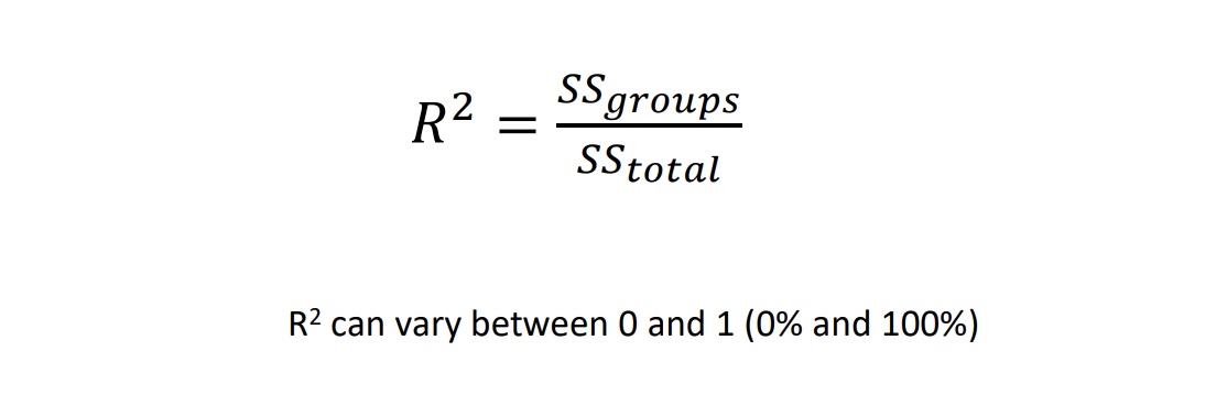
Variation explained: R 2 (“R-squared”)

ssgroups = sum of sqrs

SUMMARY OF HOW ANOVA WORKS

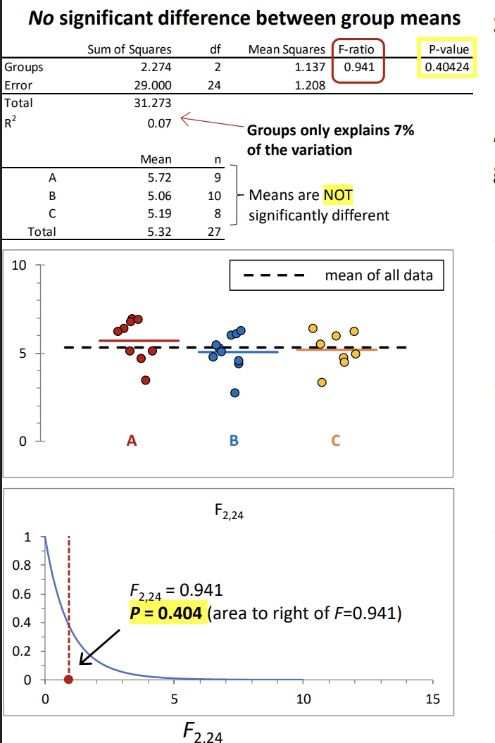
Example of an ANOVA when there is no significant difference between the group means

• F-ratio is small (expected value ≈ 1.0 under null hypothesis that mean of all groups is the same). •

R 2 is small (groups only explains a small amount of the overall variation in data)

• Large area to the right of the Fdistribution curve (P > 0.05).

The Tukey-Kramer test

Performed only if ANOVA shows a significant difference among group means

• Compares each of the group means against each other (pairwise comparisons)

When to use tukey kramer

1. You run an ANOVA

2. The ANOVA p-value is significant (p < 0.05)

This test is appropriate when:

• You’re comparing 3 or more groups

• You want to compare every possible pair of group means

• The sample sizes may be unequal (Tukey-Kramer adjusts for this)

Purpose of tukey-kramer

n R or output tables, you’ll usually see:

• A mean difference for each group pair (e.g., A vs. B)

• A confidence interval

• A p-value

➤ Interpretation rules:

Output	Meaning
p < 0.05	✅ The two group means are significantly different
p ≥ 0.05	❌ No significant difference between those two groups
CI does not include 0	✅ Significant difference
CI includes 0	❌ Not significant

---

📊 Example Scenario: tukey

📊 Example Scenario:

You test 3 diets: A, B, and C
ANOVA p-value = 0.003 → Significant → You do Tukey-Kramer

Tukey-Kramer results:

Group Pair	Mean Difference	p-value	95% CI
A vs. B	5.2	0.01	[1.2, 9.2]
A vs. C	1.1	0.45	[-2.0, 4.2]
B vs. C	4.1	0.03	[0.4, 7.8]

Interpretation:

• ✅ A vs. B and B vs. C are significantly different

• ❌ A vs. C is not significantly differen

Assumptions of ANOVA

(1) Random samples

(2) Normal distributions for each population

(3) Equal variances for all populations

Meeting the assumptions of ANOVA

1. normaility can be assessed using shapiro wilk, if not norm distrib, data may meet assumptions

2. equal variance can be assessed using levene test

3. if assumptions cannot be met, a kruskal-wallis test can be used

Kruskal-Wallis test

• Purpose: Compare 3 or more independent groups when data is not normal or assumptions for ANOVA are violated

• Data Used: Ranks (not raw values); works with ordinal or non-normal data

• H₀: All group medians are equal

• Hₐ: At least one median differs

• Interpretation:

  • p < 0.05 → Significant → At least one group differs

  • p ≥ 0.05 → Not significant → No evidence of difference

Dunn test

Nonparametric test equivalent of a Tukey-Kramer test

• Tests all the pairwise differences between groups

H0 : Median of group i = median of group j for all combinations of groups

Ha : Median of group i ≠ median of group j for all combinations of groups

Fix effects

An explanatory variable with groups that are predeterminedand of direct interest. (The thing we really want to study