psychology 2910 - lecture 13 (independent samples t-test)

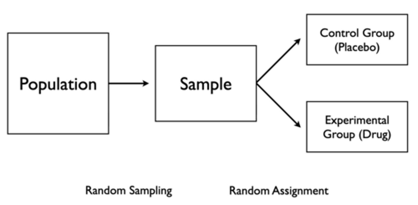
Controlled Experiment

Random sampling, then random assignment to control group (placebo) and experimental group (drug)

In-Situ Design

Randomly sampling from two groups (male and female) and distributing them into two groups (not random assignment)

How can we compare the mean of the experimental group and the mean of the control group (or the mean of Group 1 and the mean of Group 2)?

Independent t-test

Independent Groups

Participants in each group must be different, a between-subject design

- If participants are in both groups (a within-subject design); use dependent groups t-test

Normality of Dependent Variable

The sample dependent variable should be normally distributed

However, t-test is robust; correct decision will be made for minor violations (i.e. even if sample size isn't large enough)

Homogeneity of Variance

The variance of two groups will be equal or approx. equal. This assumption is important in order to create a better estimate of SD (σ) by pooling the sample SDs

How can we test for homogeneity of variance if sample sizes are unequal?

- t-test is robust if you have equal sample sizes

- If sample sizes are unequal, you can test for homogeneity of variance (Levene's F test), and if not homogenous, can use alternate procedures (different formula, transform the data)

- Only a problem if both sample sizes are unequal and homogeneity of variance is violated (we won't deal with that situation in this course!)

The logic of the independent samples t-test is the same as the one-sample t-test. You take the difference between the means, divide it by the standard error, and check it against a critical t-value defined by df.

Therefore, what is the difference between an independent samples t-test and a one-sample t-test?

- Main difference is that your standard error is not the standard error of the mean, but the standard error of the difference of means (i.e. independent samples compares means of two separate groups)

- Under null hypothesis, we would expect that our mean difference would be zero, so the t-statistic calculates how many standard errors the mean difference is from zero

Pooled Variance

A weighted average of the two sample variances. Weighted by df, not by n

16 depressed patients were randomly assigned to Prozac or Euzac conditions (double-blind). One month later, their depression score was measured (low = less depressed; high = more depressed).

How can we construct null and alternative hypotheses?

H0: μ of Prozac = μ of Euzac

Ha: μ of Prozac ≠ μ of Euzac

Assume α = 0.05

16 depressed patients were randomly assigned to Prozac or Euzac conditions (double-blind). One month later, their depression score was measured (low = less depressed; high = more depressed). The mean of the Prozac group was 68.50, and the mean of the Euzac group was 48.375.

How would we calculate the standard deviations? The pooled variance?

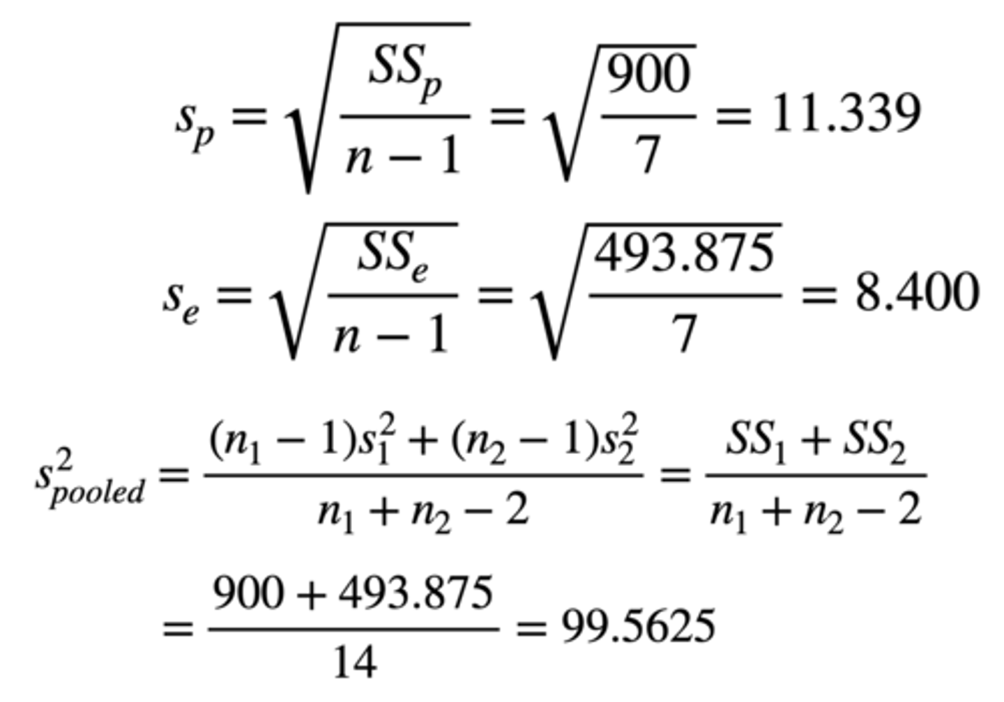
SD = √ Sum of squares / n - 1 = √ 900 / 8 - 1 = 11.339

√ Sum of squares / n - 1 = √ 493.875 / 8 - 1 = 8.400

Pooled variance = First sum of squares + second sum of squares / n1 + n2 - 2

= 900 + 493.875 / 8 + 8 - 2

= 99.5625

16 depressed patients were randomly assigned to Prozac or Euzac conditions (double-blind). One month later, their depression score was measured (low = less depressed; high = more depressed). The mean of the Prozac group was 68.50, and the mean of the Euzac group was 48.375.

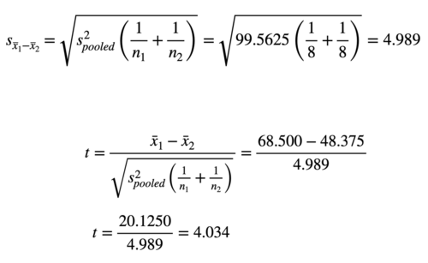
How would we calculate the standard error between the two independent sample means, then the t-test?

Standard error = √ Pooled variance (1 / n1 + 1 / n2)

= √ 99.5625 (1/8 + 1/8)

= 4.989

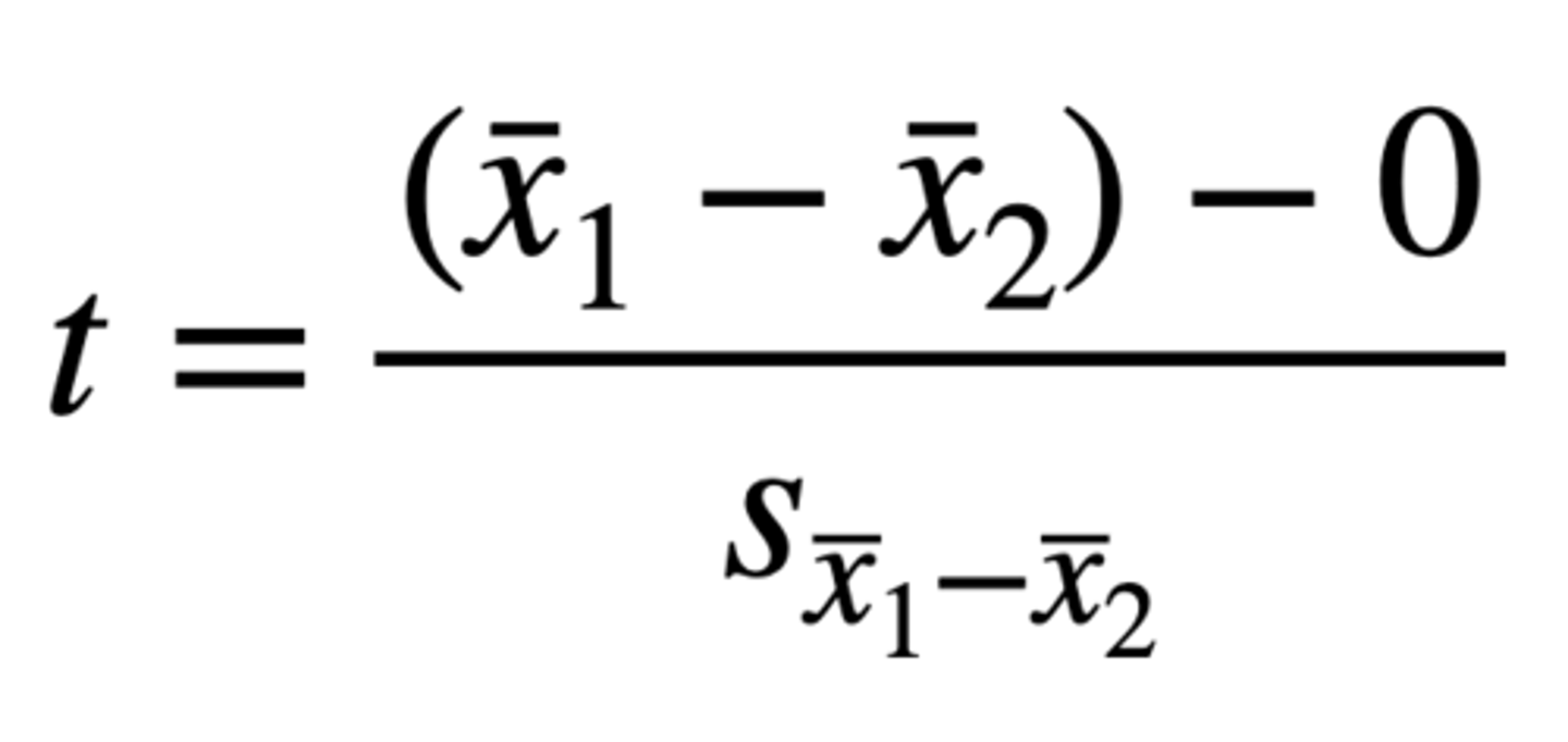
t-test = Difference between means / standard error

= 68.500 - 48.375 / 4.989

= 20.1250 / 4.989

= 4.034

16 depressed patients were randomly assigned to Prozac or Euzac conditions (double-blind). One month later, their depression score was measured (low = less depressed; high = more depressed). The mean of the Prozac group was 68.50, and the mean of the Euzac group was 48.375.

Does the calculated t-value exceed the critical t-value? What can we conclude about the hypothesis?

Calculated t-value: 4.034

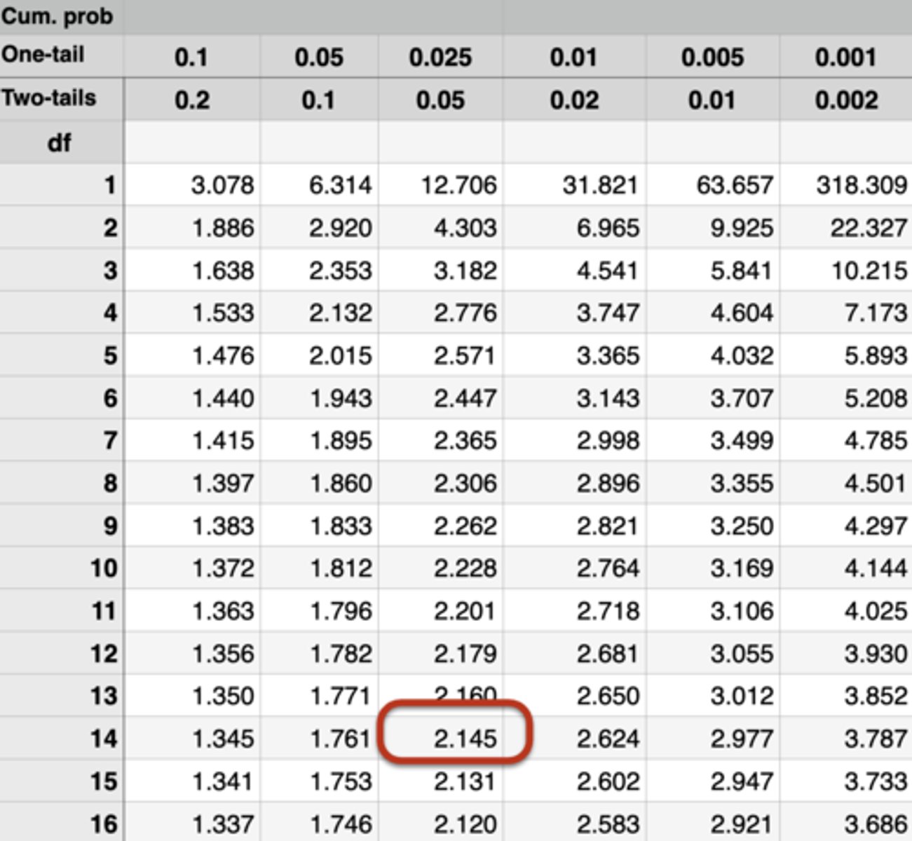
Critical t-value (look it up in table): 2.145

4.034 > 2.145; therefore, reject the null

Depressed patients who received Euzac had a significantly lower depression score (M = 48.38, SD = 8.40) than those who received Prozac (M = 68.50, SD = 11.34), t(14) = 4.034, p < .05

What if the calculated t-value were -4.034 instead of +4.034 (directional/one-tailed)?

Exactly the same as a non-directional (two-tailed) test!

- Is calculated t-value ≥ + critical t-value

- Or is calculated t-value ≤ - critical t-value

What is the difference between a two-tailed and one-tailed test?

Two-tailed:

- More conservative

- Less likely to result in Type I Error

- More likely to miss a real (but small) difference

One-tailed:

- More liberal

- More sensitive to real (but small) differences

- Also more likely to result in Type I Error

Should we typically conduct a one- or two-tailed test?

Use non-directional (two-tailed) test unless you have a compelling reason to do otherwise

- Will have difficulty convincing reviewers/editors that one-tailed is genuine

- Bias is to view one-tailed test as last attempt to change a non-significant result into a significant result

- Two-tailed critical t-value might be 2.306 (not significant), whereas one-tailed critical t-value might be 1.860 (significant). Calculated t-value is 2.141 for both

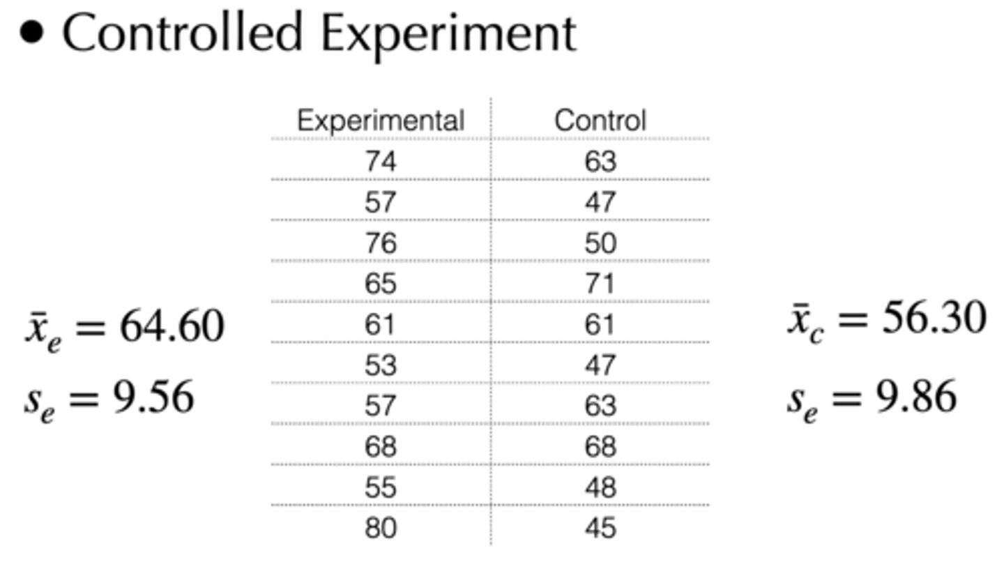
If we have the mean and standard deviation of both the control and experimental group (both counts are n = 10), then how can we construct a null and alternative hypothesis for a two-tailed test?

Experimental mean = 64.60

Experimental SD = 9.56

Control mean = 56.30

Control SD = 9.86

H0: μ of experimental group = μ of control group

Ha: μ of experimental group ≠ μ of control group

Assume α = 0.05

How can we calculate the pooled variance of the control and experimental group if we know the mean and standard deviation of each?

Experimental mean = 64.60

Experimental SD = 9.56

Control mean = 56.30

Control SD = 9.86

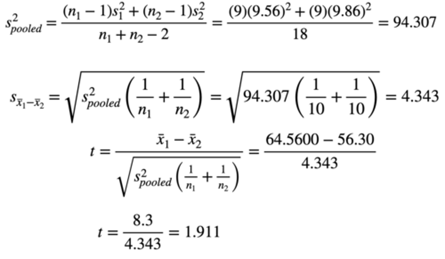
Pooled variance = First sum of squares + second sum of squares / n1 + n2 - 2

= (9)(9.56)^2 + (9)(9.86)^2 / 18

= 94.307

How can we calculate the standard error between the control and experimental group if we know the mean and standard deviation of each? How can we conduct a t-test?

Experimental mean = 64.60

Experimental SD = 9.56

Control mean = 56.30

Control SD = 9.86

Standard error = √ Pooled variance (1 / n1 + 1 / n2)

= √ 94.307 (1/10 + 1/10)

= 4.343

t-test = Difference between means / standard error

= 64.60 - 56.30 / 4.343

= 8.3 / 4.343

= 1.911

Does the calculated t-value exceed the critical t-value? What can we conclude about the hypothesis?

Experimental mean = 64.60

Experimental variance = 9.56

Control mean = 56.30

Control variance = 9.86

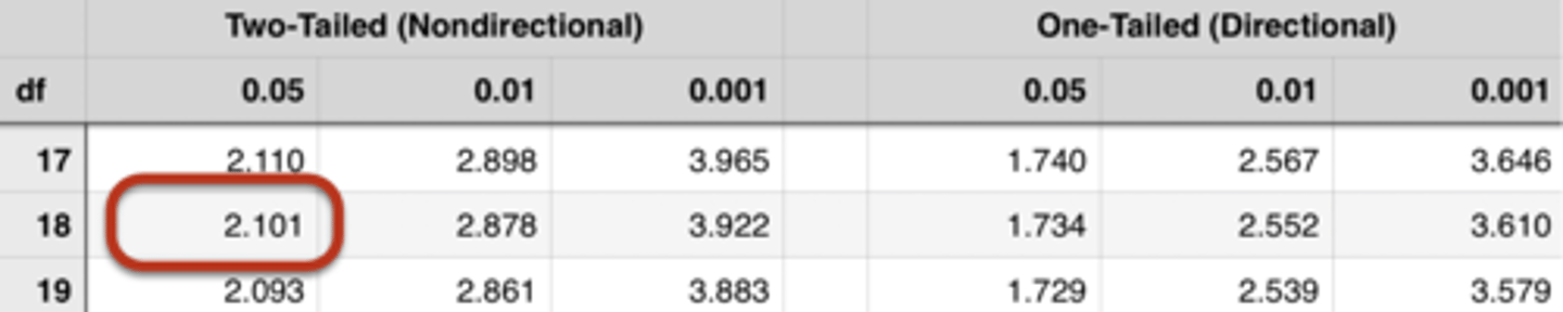
Degrees of freedom: 10 + 10 - 2 = 18

Calculated t-value: 1.911

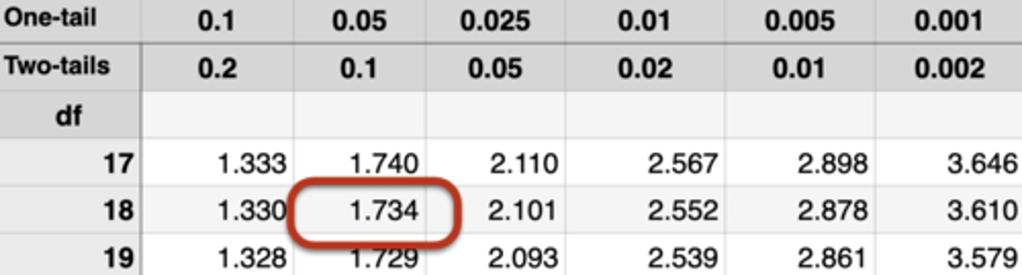
Critical t-value: 2.101 (two-tailed test, α = 0.05, df = 18)

We cannot reject the null!

Although subjects in the experimental group scored slightly higher (M = 64.60, SD = 9.56) than those in the control group (M = 56.30, SD = 9.86), this difference was not significant using a two-tailed test, t(18) = 1.911, p > .05

If we have the mean and standard deviation of both the control and experimental group (both counts are n = 10), then how can we construct a null and alternative hypothesis for a one-tailed test?

Experimental mean = 64.60

Experimental SD = 9.56

Control mean = 56.30

Control SD = 9.86

H0: μ of experimental group ≤ μ of control group

Ha: μ of experimental group > μ of control group

Assume α = 0.05

Does the calculated t-value exceed the critical t-value in a one-tailed test (compared to the two-tailed test)? What can we conclude about the hypothesis?

Experimental mean = 64.60

Experimental variance = 9.56

Control mean = 56.30

Control variance = 9.86

Degrees of freedom: 10 + 10 - 2 = 18

Calculated t-value: 1.911

Critical t-value: 1.734 (one-tailed test, α = 0.05, df = 18)

We reject the null!

Subjects in the experimental group scored higher (M = 64.60, SD = 9.56) than those in the control group (M = 56.30, SD = 9.86), and this difference was significant using a one-tailed test, t(18) = 1.911, p < .05