ERE week 2 - Market instruments & dynamic efficiency

The problem with pollution

Its a negative externality

Coase theorem not applicable to most enviro problems

Govt has to intervene

Direct / command & control regulation

Control firms output of negative externalities via laws and regulations - Govt in control

• Tell firms by how much (and how) to reduce pollution

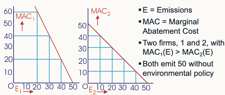
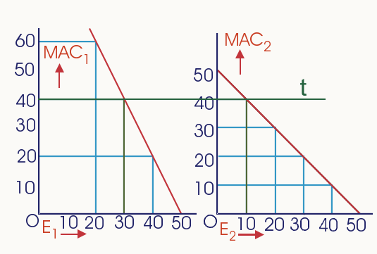
2 firm pollution diagram

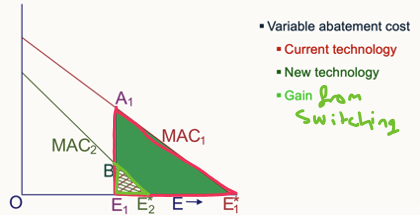
Reducing emissions costs firms → Cheapest emission reduction methods used first but get increasingly more expensive

2 firm pollution diagram - Govt caps firm emissions

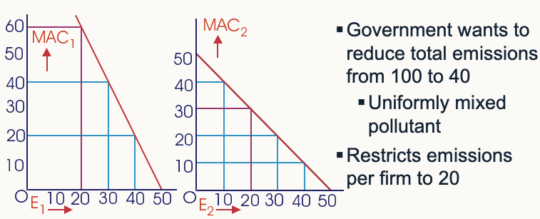
Uniformly mixed pollutant

Damage from pollutant doesn’t depend on where the emissions are

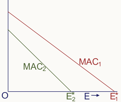
2 firm pollution diagram - Optimal pollution

Lower MAC for firm 2 - optimal for it to pollute less

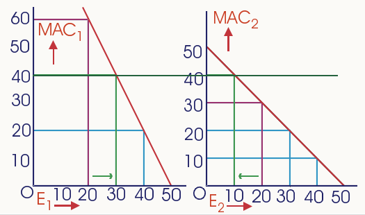
Optimal pollution level

Where MACs are equal

minimises overall costs

Problems with optimal / efficient pollution for Govt

Need to know firms individual MAC

Firms don’t have incentive to find out and disclose

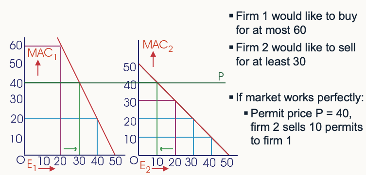
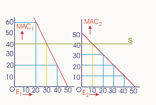
Tradable emission permit system

The govt allocates permits for both firms to emit a certain level of E but the firms can trade them

2 firm pollution diagram - Tradable permits

Govt allocates permits for both to emit 20 (wants E = 40)

Cheaper for 2 to cut E so they sell permits

2 sells permits until MAC₁ = MAC₂ = permit price

How to introduce tradable permits

Grandfathering - Distribute permits for free among incumbent firms

Auction - permits sold to highest bidder

Trading results in the efficient permit allocation, whatever the initial distribution

2 firm pollution diagram - Emissions taxation

Firms choose between paying tax and abatement (reduces T paid)

Set MAC = T

Each firm has different E & T

2 firm pollution diagram - Abatement subsidy

Firm paid to reduce emissions below a baseline

Firms reduce emissions till subsidy rate (s) = MAC

• past s its more expensive to reduce emissions than you gain from the subsidy

Costly to Govt

Market instruments vs Direct regulation

Market:

• Govt only needs to know aggregate MACs

• Tradable - Emission target always met if cap enforced

  • Costs not known in advance

• Tax - Emissions may be above or below target

  • MAC known in advance

Direct

• less cost effective

Are permit trading outcomes independent of allocation?

Theory - Permit trading leads to efficient allocation whatever initial allocation

Can use initial distribution for political means – most permits to firms that lobby

Strong correlation between initial allocation and ultimate emissions - TC and regulatory uncertainty? CORRELATION ≠ CAUSATION

RECLAIM programme example - overview

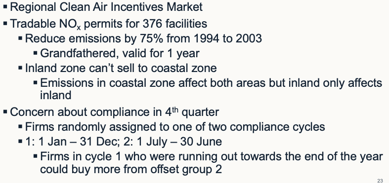
RECLAIM programme example - TC & regulatory uncertainty

• Firms had to learn about programme, abatement costs and how it works

• Broker fees to buy through a broker (1-3%)

• Questionable broker practices as well – brokers never sourced the permits

RECLAIM programme example - Allocation & E overtime

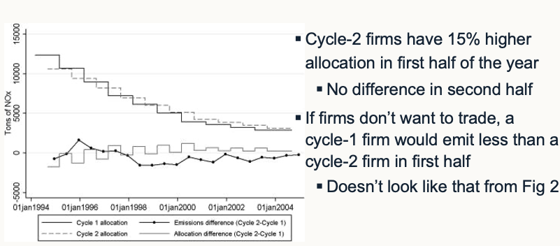
RECLAIM programme example - Empirical test (does allocation affect E)

Dependent variable - Log E (per firm + per 6 months)

Explanatory variable - Initial permit allocation

Results - Only explan var (0.79***) OR Include final allocation (0.65***) OR include wage and PPI (0.65***)

Initial permit allocation affects E

RECLAIM programme example - Instrumental variables

Maybe firms exploit the existence of 2 cycles - If random assignment then cycle 2 firms no higher E

Regress allocation on Time & Fixed effects + cycle dummy

• allocation no longer significant

Empirical findings are consistent with, but not proof of, independence property

Uncertainty about abatement costs

Tradable permits

• Certainty about reaching emissions target – emissions are valuable and firms want to maximise production

• Uncertainty about costs - More / less permits should be issued if cost higher / lower than expected

Taxation

• Uncertainty of reaching emissions target - If abatement costs higher than expected, then emissions higher than expected – higher tax rate needed

• Certainty of what MAC - Firms set MAC = t

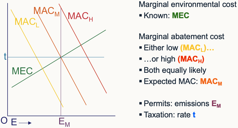
Taxes vs permit diagram - initial diagram

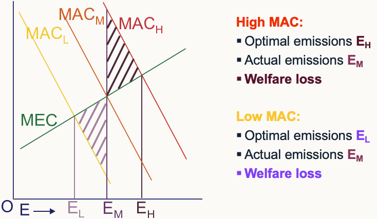
Taxes vs permit diagram - permits

Too many or too few permits issued

Total welfare loss = ½ of high welfare loss + ½ low welfare loss

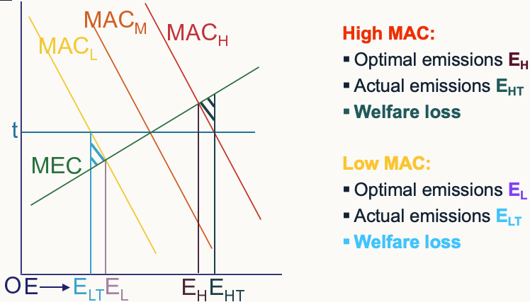
Taxes vs permit diagram - tax

Optimal emissions is different to where firms optimally choose

Firms choose where t = MAC

Social optimal is where MEC = MAC

Taxes vs permit diagram - comparison

Optimal depends on slope of MAC and MEC

• When MAC steeper than MEC – taxes better

MEC uncertain for both methods unlike MAC

Spatial dimension theory - overview

Assumptions

• 1 & 2 have same MAC

• Environmental damage function same in A & B

Spatial dimension theory - tax

Same tax rate for both firms

• BUT 1 does more damage so should have higher tax rate optimally

  • All E from 1 ends up in A or B

  • If worked out then you might as well impose direct regulation and so all benefits lost of market

Spatial dimension theory - permits

1-to-1 trade

• Both firms emit same amount

• Too much pollution from 1 in A & B

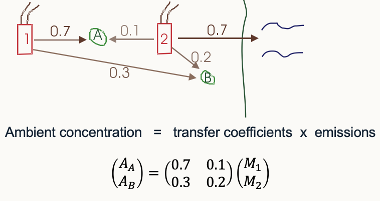
Ambient permits

• Permits used in term of conc at receptor point A or B

  • Firm 1 wants to increase emissions by 10: Needs 7 permits for A, 3 for B

• Lower administrative cost than taxation - set E cap and let firms trade

• Higher TC

• Not yet tried in real life

US air pollution example - overview

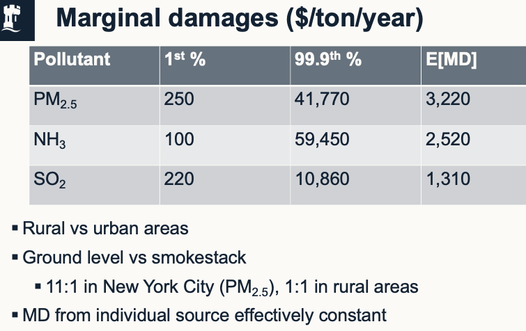
Pollutants captured from 10k point sources (country aggregated ground sources)

Source-receptor matrices give county-level concentrations

Exposures = concentration x populations (people, crops etc.)

Damages - Market price, Human health, valuation studies

US air pollution example - Marginal damages

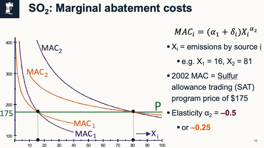
US air pollution example - SO₂ marginal abatement costs

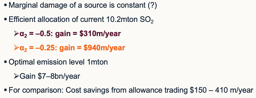
US air pollution example - Welfare gains

Dynamic efficiency

Incentive to do R&D into and adopt new technologies

→ New tech lowers E

Dynamic efficiency graph - initial

Dynamic efficiency graph - Direct regulation (E₁)

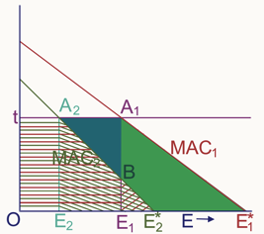
Dynamic efficiency graph - Tax / auctioned permits

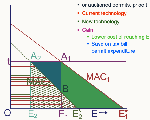
Dynamic efficiency graph - Tax / auctioned permits

Dynamic efficiency graph - Direct vs market

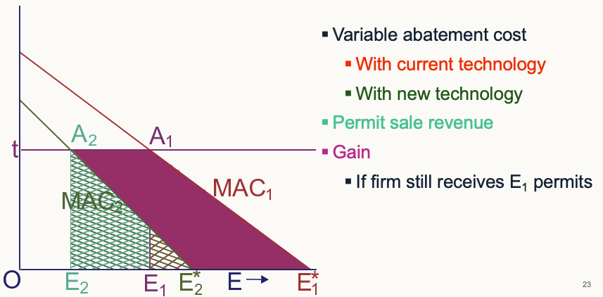
Market instruments have additional gain of net saving on tax bill / permit expenditure

• Reducing emissions to E2 gives higher abatement cost (area below MAC2)

• More than compensated by saving in tax bill

Dynamic efficiency graph - Grandfathered permits

With new tech still get E1 permits → Can sell excess at price t

Regulator may see the switch to new tech and give firm E2 permits in the future → Reduces incentive to switch

Dynamic efficiency graph - Abatement subsidy

Firm paid D → Paid more by reducing E

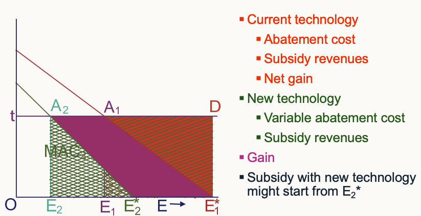
Dynamic efficiency summary

E tax + Auctioned permits give highest incentives for new technology adoption

Abatement subsidies + grandfathered permits also give these incentives (if baseline remains the same)

These high incentives for adoption are optimal

New technologies make it worthwhile to reduce emissions further - Firms should be rewarded for this gain