the firm and profit max

total cost function

relationship of a firms total costs and quantity of output

includes → fixed cost, variable cost and opportunity cost

increasing and convex function (marginal cost rises with output)

exogenous variables/shocks

‘generated outside the model’

variable is exogenous when its value is set by the modeller rather than being determined by the model itself

exogenous shock = a change in exogenous variables in a model (variables that are otherwise held constant by the modeller)

endogenous variable

‘generated by the model’

value is determined by the working of the model (rather than being set by the modeller)

the market for a differentiated product (monopoly)

differentiated product = lack of substitutes

demand curve reflects consumers willingness to pay but demand is inelastic due to lack of available substitutes

firm has market power and acts as a price setter in the market

isoprofit curve

curve that joins together the combinations of prices and quantities of a good that provide equal profits to a firm

equivalent to the firms indifference curve → want to produce on the highest isoprofit curve

same shape as the AC curve (if firm produces on an isoprofit curve above AC curve its making profit)

slope of isoprofit curve = (P - MC) / Q

equation for isoprofit curve in (Q, P) plane is P = C(Q)/Q + k/Q

• where k is a constant level of profiit

scale of production

economies of scale → when a firm is experiencing increasing returns to scale when it increases output (increase in output is proportionally greater than increase in inputs)

diseconomies of scale → when a firm is experiences decreasing returns to scale when it increases output (increase in output is proportionally less than increase in inputs)

consumer surplus

surplus equal to willingness to pay - the price

consumer surpluses is the sum across all consumers

producers surplus

producer receives a surplus on each unit = price - marginal cost of producing it

producer surplus refers to the sum across all units sold

profit = producer surplus - fixed costs

gains from trade

producer surplus + consumer surplus

gains from trade are maximsied when there is no DWL

highest gains from trade is where demand curve intersects the highest isopofit curve

deadweight welfare loss calculation

measurement of the total loss of surplus (gains from trade not exploited) relative to the maximum available in the market

• derive P*, Q* from profit max problem

• compute MC(Q*)

• base of triangle = P* - MC(Q*)

• find Pareto efficient point by solving P(Q) = MC(Q)

• height of triangle = Pareto efficient point - Q*

• work out triangle

price markup

price - MC / price

proportion of the price

markup is inversely proportional to the elasticity of demand for the good at that price

profit maximisation calculation for price setting firms

firms wants to reach highest isoprofit curve whilst being limited by demand (feasible frontier)

• define TR as TR = P(Q) x Q

• substitute the inverse demand expression P(Q) into R(Q)

• differentiate with respect to Q to get MR

• differentiate TC with respect to Q to get MC

• set MR = MC to find Q*

• substitute Q* into P(Q) to find P*

• verify profit is maximised by checking second order condition → negative second order derivative shows that profit function is concave

point of profit max is MR = MC which is TR’ = TC’

market with homogenous products (perfect competition)

elastic demand curve as there are lots of substitutes available

competitive equilibirum → firms are price takers as there are many buyers and sellers with perfect information

Pareto efficient if there are no externalities

demand and marginal revenue

change in total revenue from selling one more unit of output

• gain from selling one more unit at a new price

• loss from lowering the price of the intra-marginal units

PED

% change in demand / % change in price

the higher the slope of the inverse demand, the lower the elasticity of demand

PED and MR

if demand is elastic → reducing price will lead to a large rise in quantity and total revenue will increase

if demand is inelastic → reducing price will lead to a small rise in quantity and total revenue will fall

profit maximisation for price taking firm

P* = MC

firms supply curve = MC curve (market supply is the sum of all the MC curves)

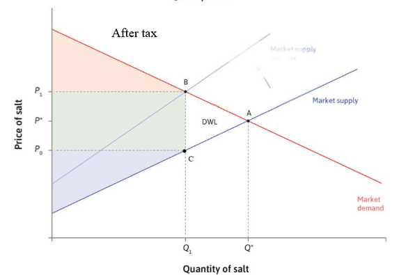
effects of taxes in price taking market

• supply curve shifts upwards

• consumers pay more (P* to P1)

• producers recieve less (P* to P0)

• quantity falls (Q* to Q1)

total surplus = consumer surplus + producer surplus + government revenue

model with externalities

MPC → producers cost of producing one more unit

MEC → the extra cost of producing one more nit borne by others

MSC → MPC + MEC

power rule

nx^n-1

function for total revenue

inverse demand function x Q

how to compute profit margin

base of the triangle for DWL (gap between MC(Q*) and P*

profit margin = P* - MC (Q*)

quantity efficiency gap

gap between Pareto efficient output point and Q*

how to get market supply from MC

add Q/number of firms to q in MC function

then divide number attached to q by number of firms

eg MC = 2 + 16q and number of firms is 20

Ps = 2 + 16(Q/20)

Ps = 2 + 0.8Q