Microbial Genetics Part III - Molecular Diagnosis

1. history and physical

2. biological specimen

3. phenotype-based diagnosis methods

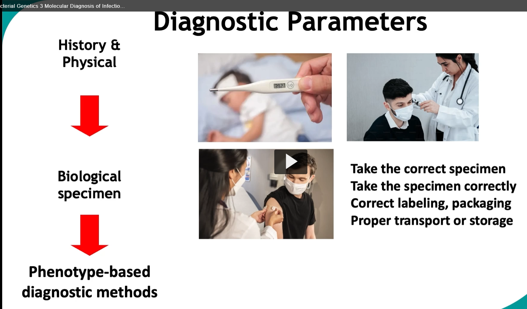
in diagnosing infections, we start with the gram stain:

4. microscopy gram stain

5. culture biochemical testing (agar or broth, help reach a definitive diagnosis)

6. antibiotic sensitivity (uses discs with various antibiotics in the agar plate to find the most effective treatment)

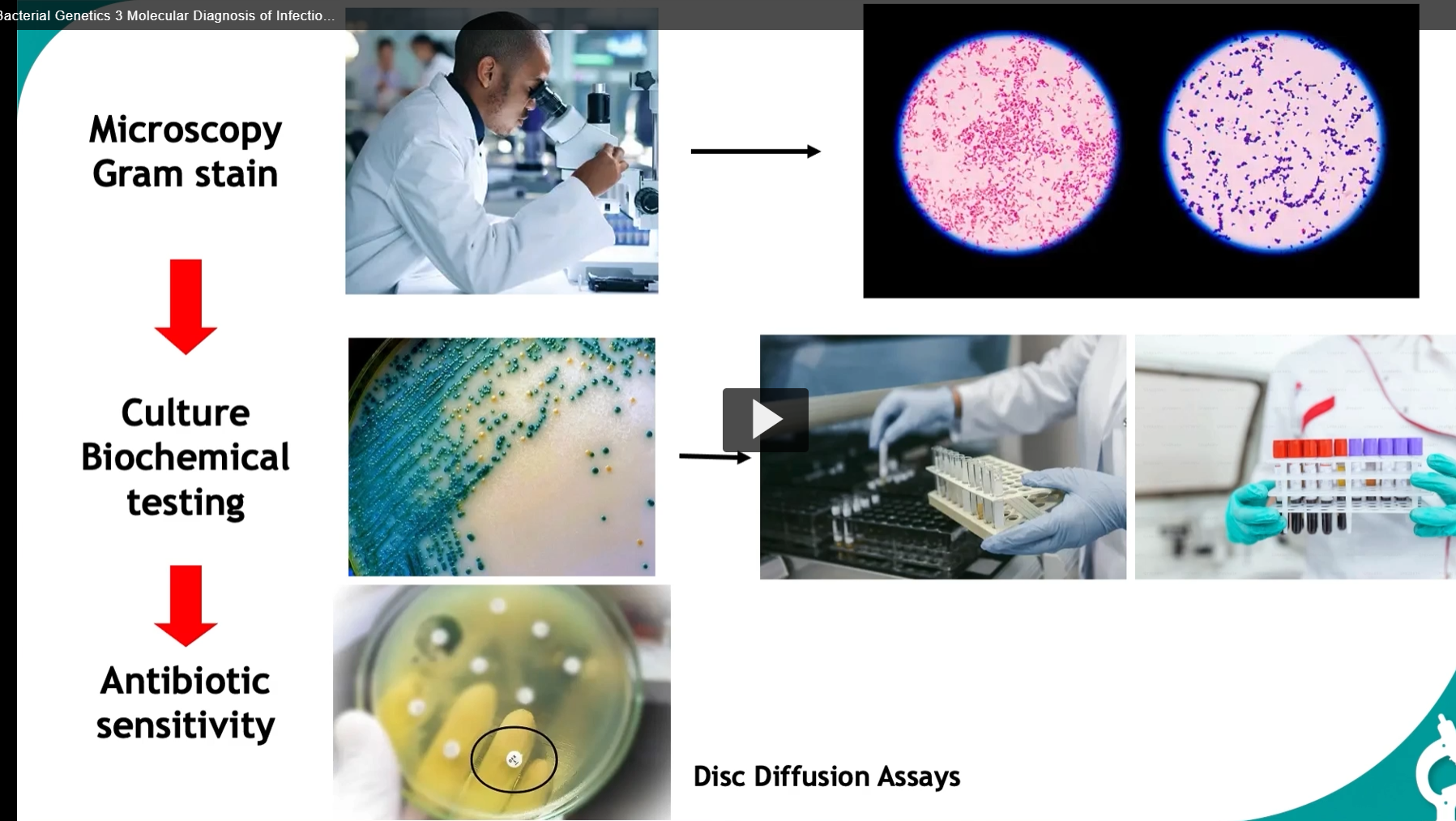
Serology (antigen/antibody detection)

-serology mechanisms for available for identifying infectious organisms.

This approach is based on the detection of antibodies produced in response to an infectious agent, or for the detection of epitopes from circulating antigens from the agent in the patients serum.

1. Eliza (useful for quantifying the presence of antibodies or antigens in a sample)

2. Immunofluorescence (can visually demonstrate the presence of specific antigens or antibodies by labeling them with a fluorescent dye.

3. Agglutination

4. Use of monoclonal and polyclonal antibodies in Western Blot (western blot is shown here and is particularly used for confirming the presence of proteins associated with certain infections).

In a western blot test, proteins are separated by gel electrophoresis and then transferred to a membrane where they are probed with antibodies that are specific to the target antigen. If the target antigen is present, it will bind to the specific antibody, which can then be detected often through a color change.

ELISA — Definition & Etymology

Definition:
ELISA stands for Enzyme-Linked Immunosorbent Assay.
It is a laboratory technique used to detect and quantify specific antigens or antibodies in a sample (e.g., blood, serum). It works by using antibody–antigen specificity and an enzyme-driven color change as a readout.

Etymology (break it down)

• Enzyme

  • en- = “in”

  • zyme (Greek zymē) = “ferment, yeast”
    → A molecule that drives biochemical reactions

• Linked
  → The enzyme is attached (linked) to an antibody

• Immuno-

  • Latin immunis = “exempt, protected”
    → Refers to the immune system

• Sorbent

  • Latin sorbere = “to absorb or suck in”
    → The assay uses a surface that binds (absorbs) molecules

• Assay

  • Old French assai = “trial, test”
    → A test or analytical procedure

Put together: “A test where immune molecules are captured on a surface and detected using an enzyme-linked signal.”

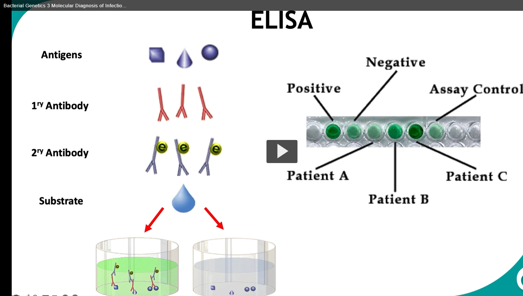
What’s happening in the diagram (step-by-step)

This slide shows a typical indirect ELISA workflow:

---

1. Antigen is present (top row)

• Different shapes = different antigens (targets you’re trying to detect)

2. Primary antibody (1° antibody) binds antigen

• The primary antibody is specific to the antigen

• If the antigen is present → antibody binds

• If not → nothing binds

3. Secondary antibody (2° antibody) binds the primary

• The secondary antibody recognizes the primary antibody

• It is enzyme-linked (the yellow “e” in the diagram)

• This step amplifies the signal (more enzymes per antigen)

4. Substrate is added

• A substrate (colorless chemical) is added

• The enzyme converts it into a colored product

5. Color change = positive result

• Green color → Positive
  → Antigen was present → full antibody chain formed → enzyme reaction occurred

• Clear/no color → Negative
  → No antigen → no enzyme → no reaction

---

🧪 Interpreting the plate (right side)

• Patient A → dark green → strong positive

• Patient B → lighter green → weaker positive (lower concentration)

• Patient C → no color → negative

• Assay control → ensures the test is working properly

---

Conceptual takeaway (important for exams)

ELISA is essentially: “Convert invisible molecular binding into a visible color signal.”

• Specificity → antibody–antigen binding

• Sensitivity → enzyme amplification

• Readout → color intensity ∝ amount of target

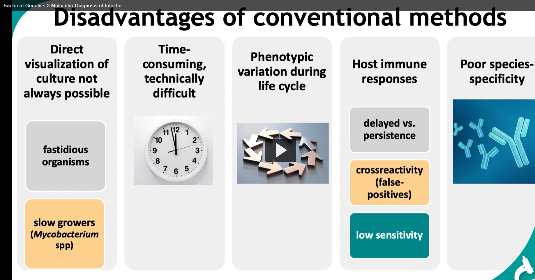
Disadvantages of conventional methods

Direct visualization of culture not always possible

• fastidious organisms

• slow growers (Mycobacterium spp)

---

Time-consuming, technically difficult

---

Phenotypic variation during life cycle

---

Host immune responses

• delayed vs. persistence

• crossreactivity (false-positives)

• low sensitivity

---

Poor species-specificity

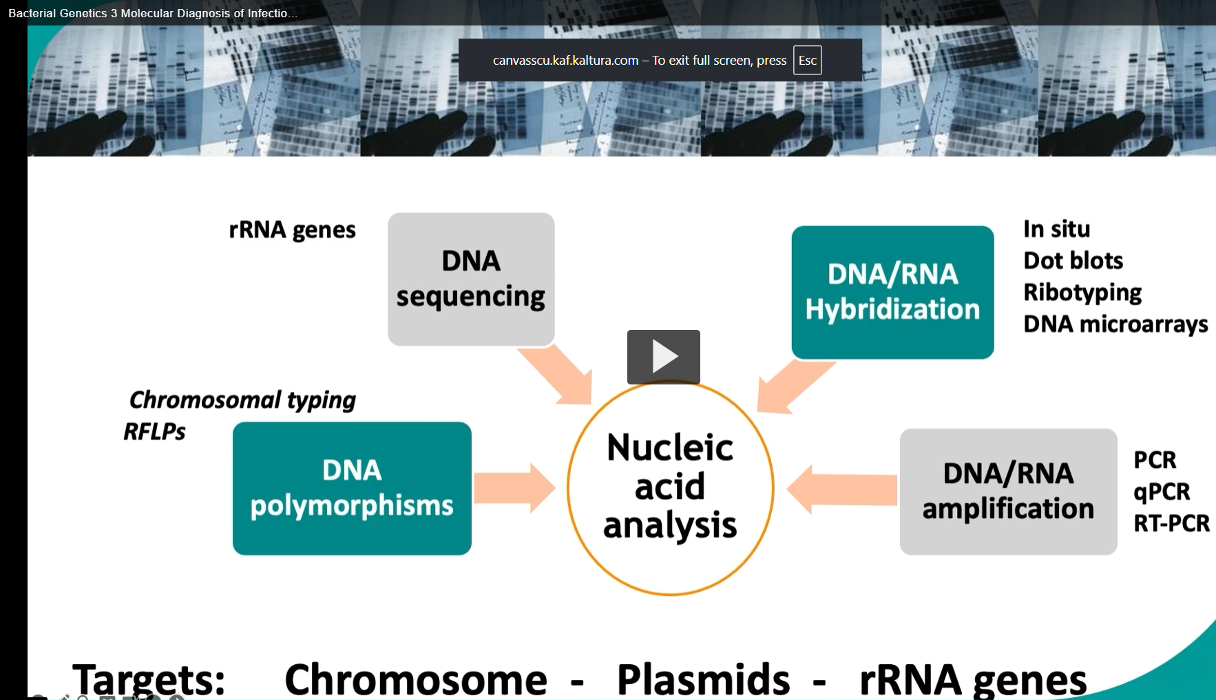
Genotype based tests that analyze DNA or RNA overcome traditional diagnostic limitations by identifying microbial pathogens through genetic variations using methods like restriction fragment length, polymorphism, RFLP, and specific hybridization probes.

DNA sequencing, especially of the 60S ribosomal RNA genes, offers precise organism identification.

For samples with low nucleic acid levels, amplification techniques like PCR or RT PCR boost sensitivity and specificity, enabling the detection of minute quantities of genetic material. Potential targets for these techniques include genomic DNA of the bacterial chromosome, plasmids, such as R factors, and ribosomal RNA genes

By exploiting the unique characteristics of these genetic materials, laboratory professionals can accurately identify microorganisms, understand their resistance mechanisms, and guide the appropriate treatment strategies.

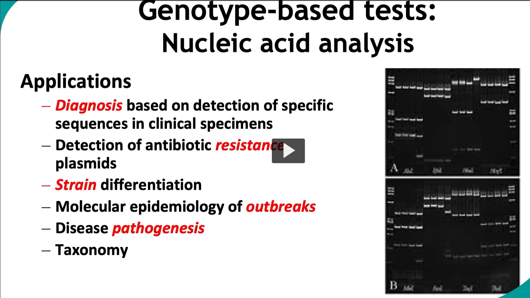
Genotype-based tests: Nucleic acid analysis

---

Applications

• Diagnosis based on detection of specific sequences in microbial pathogens from the patient, environment, or culture samples.

• Key applications: Detection of antibiotic resistance plasmids (vital for outbreak management in healthcare settings)

• These techniques allow for precise Strain differentiation

• Molecular epidemiology of outbreaks, helping trace infections, sources, and spread.

• Provide insights of Disease pathogenesis and microbial evolution.

• Taxonomy

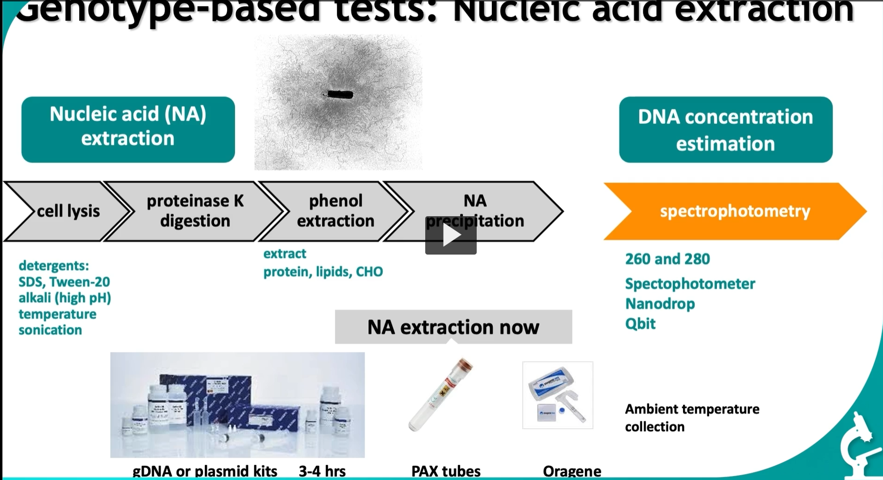
we extract nucleic acids (DNA/RNA) from cells and then measure how much we got.

Think of it as: “Break cells → isolate DNA → measure DNA quality & quantity.

1: Nucleic Acid Extraction (left side)

1. Cell lysis = breaking open the cell

Goal: release DNA from inside the cell

Methods listed:

• Detergents (SDS, Tween-20) → dissolve cell membrane (lipids)

• Alkali (high pH) → destabilizes membranes and proteins

• Temperature → helps break structures

• Sonication → sound waves physically disrupt cells

Concept: You’re destroying the “container” (cell membrane + nucleus) to access DNA.

2. Proteinase K digestion

Goal: remove proteins

• Proteinase K is an enzyme that digests proteins (to remove them)

• It removes:

  • histones (DNA-binding proteins)

  • enzymes that could degrade DNA

Concept: DNA is “wrapped in protein”—you must remove proteins to purify it.

3. Phenol extraction: separate DNA from other biomolecules

• Phenol separates:

  • Proteins → organic layer

  • DNA → aqueous layer

Slide note:

• “extract protein, lipids, CHO (carbohydrates)”

→ Concept: This is a chemical separation step—like oil and water layers.

4. Nucleic Acid (NA) precipitation: pull DNA out of solution

• Add alcohol (ethanol/isopropanol) → DNA becomes insoluble

• DNA forms a visible pellet

→ Concept: Turning dissolved DNA into a solid you can collect

5. Collected by centrifugation

6. the purity and concentration of DNA is assessed by spectrophotometry with absorbance ratios between 1.8 and 2.0 indicating HIGH PURITY.

Part 2: DNA Concentration Estimation (right side)

After extraction → you must check:

1. How much DNA?

2. How pure is it?

---

Spectrophotometry

Measures how much light DNA absorbs.

Key wavelengths:

• 260 nm → DNA absorbs here

• 280 nm → proteins absorb here

Ratio (important!):

• 260/280 ≈ 1.8 → pure DNA

• Lower → protein contamination

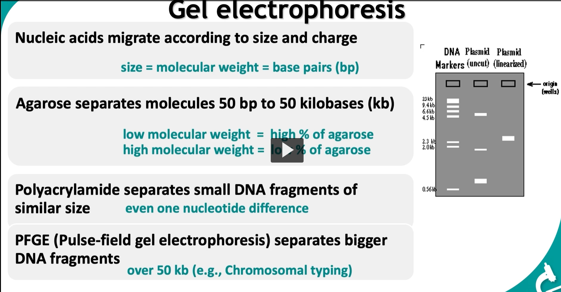
AFTER, DNA extraction, the next step is assessing nucleic acid quality and fragment size.

Gel electrophoresis: using electricity (electrophoresis) to separate DNA based on size AND charge.

Why DNA moves

• DNA has a negative charge (because of phosphate groups)

• When electricity is applied:

  • DNA moves toward the positive electrode

What determines movement? 1. Size (most important)

• Smaller fragments → move faster → travel farther

• Larger fragments → move slower → stay near the top

That’s why: Distance traveled ∝ inverse of size

The gel = molecular sieve

Think of the gel like a mesh/net:

• Small DNA → slips through easily

• Large DNA → gets slowed down

different types of gels

Agarose gel (most common) Range:

• Separates ~50 bp to 50 kb

Key concept:

• Higher % agarose → tighter mesh → better for small DNA

• Lower % agarose → looser mesh → better for large DNA

Easy memory: Tight gel= small DNA

Polyacrylamide gel

Used for:

• Very small fragments

• Can detect 1 nucleotide difference

→ Much higher resolution than agarose

Used in:

• sequencing

• SNP analysis

PFGE (Pulse-Field Gel Electrophoresis)

• Very large DNA (>50 kb)

How it works:

• Electric field changes direction periodically

• Forces large DNA to reorient and separate

→ Used in: chromosomal typing

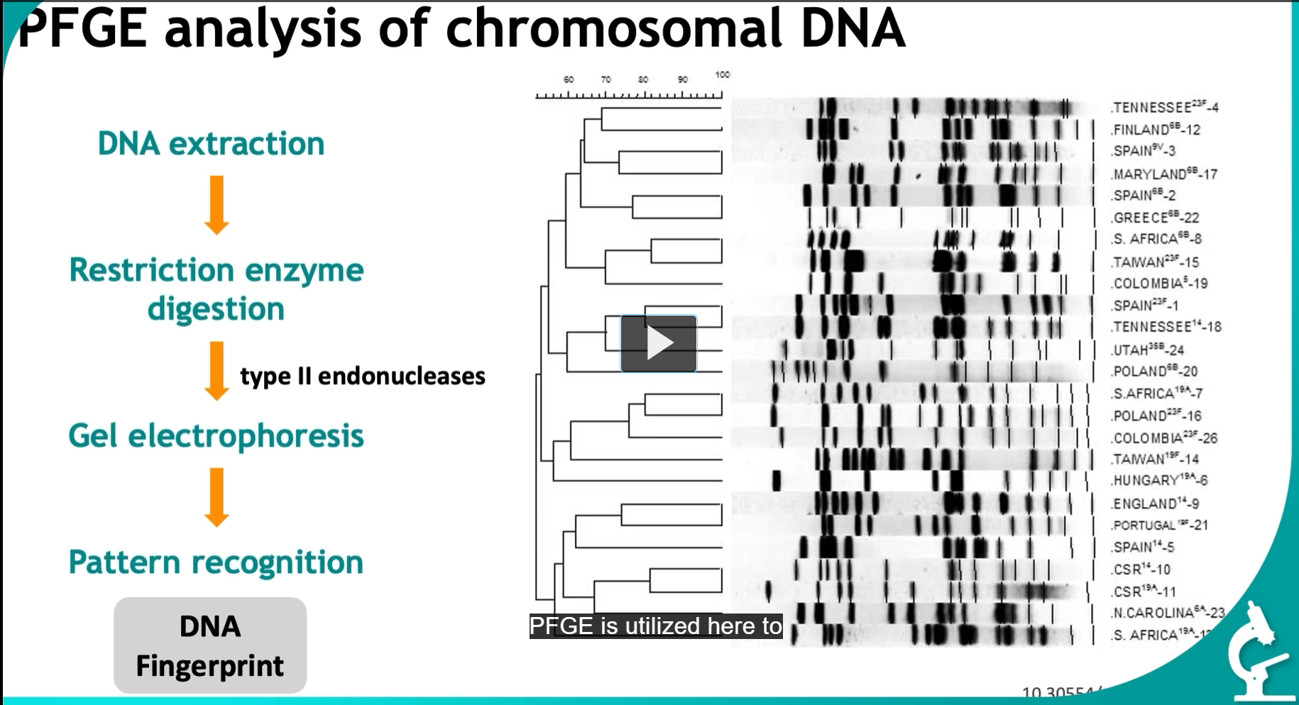
PFGE analysis of chromosomal DNA (from tracking infections)

---

DNA extraction (taken from isolates from various hospital areas)
↓
Restriction enzyme digestion

• type II endonucleases (Cut DNA at specific sequences, Produce large DNA fragments
  ↓
  Gel electrophoresis (This is NOT normal gel electrophoresis, (PFGE specifically)
  ↓
  Pattern recognition (by comparing the resulting patterns, this is called a DNA fingerprint, we can identify the presence of the same organisms, crucial for understanding the presence of the same organism, crucial for understanding the spread of infections

when DNA is digested with restriction enzymes, this process is known as RESTRICTION, FRAGMENT LENGTH POLYMORPHISM.

This technique targets specific DNA sequences that are unique to an organism, creating a distinctive fingerprint, useful for diagnostics.

The process involves:

1. isolating DNA

2. digesting it with restriction enzymes

3. separating the resulting fragments using agarose gel electrophoresis.

to enhance specificity, probes can hybridize conserved regions of the DNA, providing precise identification.

4. In this example, we use RFLP to differentiate between three bacterial strains,

we isolate

1. chromosomal DNA

2. digest it with type II endonucleases

3. and separate the fragments by gel electrophoresis.

4. Specificity is enhanced by hybridizing the specific probe that identifies the DNA fragment.

5. The results show that strains I and II are identical while strain III is a different bacterium. (strain III is at a different position)

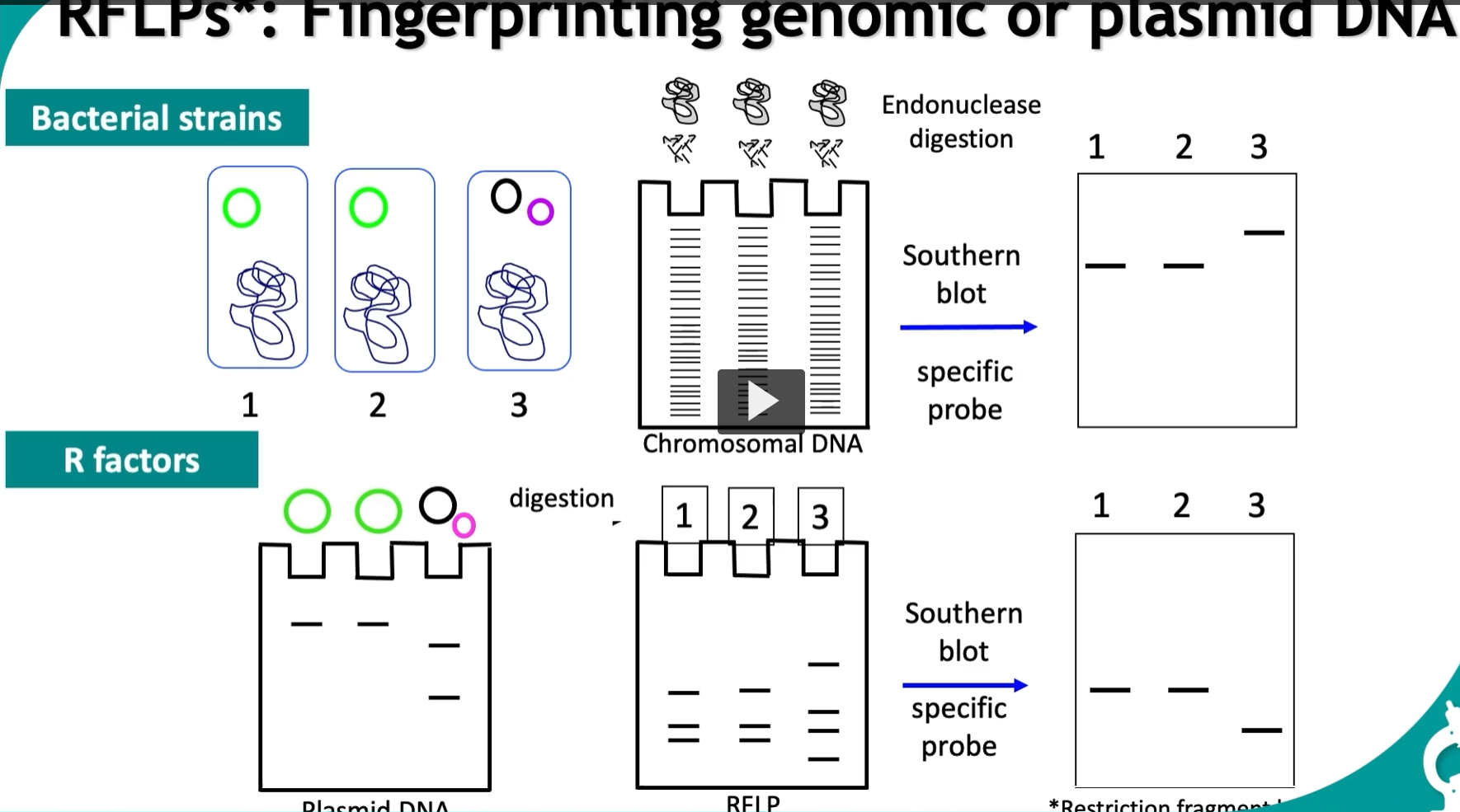
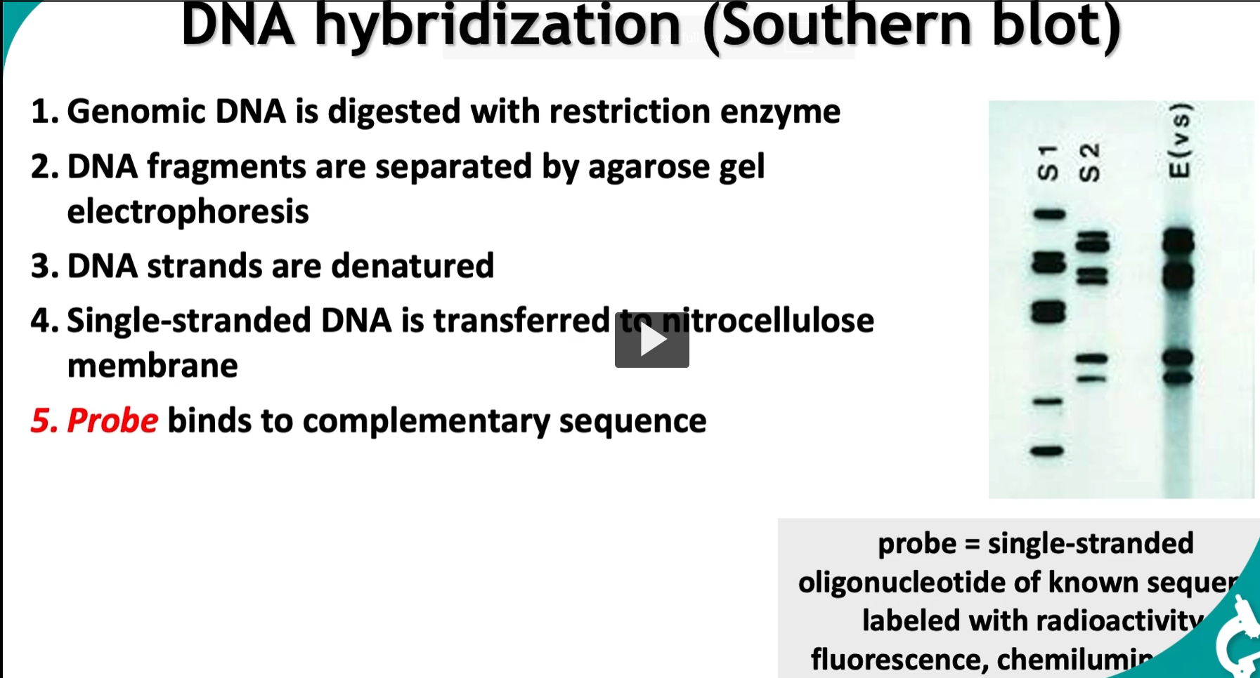
DNA hybridization (Southern blot)

Southern blot = find a specific DNA sequence by using a complementary labeled probe.

“Cut DNA → separate → transfer → detect with a probe.”

---

1. Genomic DNA is digested with restriction enzyme (These enzymes recognize specific sequences and cut DNA into fragments, A mixture of many DNA fragments of different sizes)

2. DNA fragments are separated by agarose gel electrophoresis (most common gel)

3. DNA strands are denatured

4. Single-stranded DNA is transferred to nitrocellulose membrane (The membrane is stable and accessible for probing, “Copy the gel pattern onto a durable sheet”)

5. Probe binds to complementary sequence (labeled (radioactive, fluorescent, or chemiluminescent), Probe binds ONLY where the matching sequence exists)

probe: single-stranded oligonucleotide of known sequence labeled with radioactivity, fluorescence, chemiluminescence

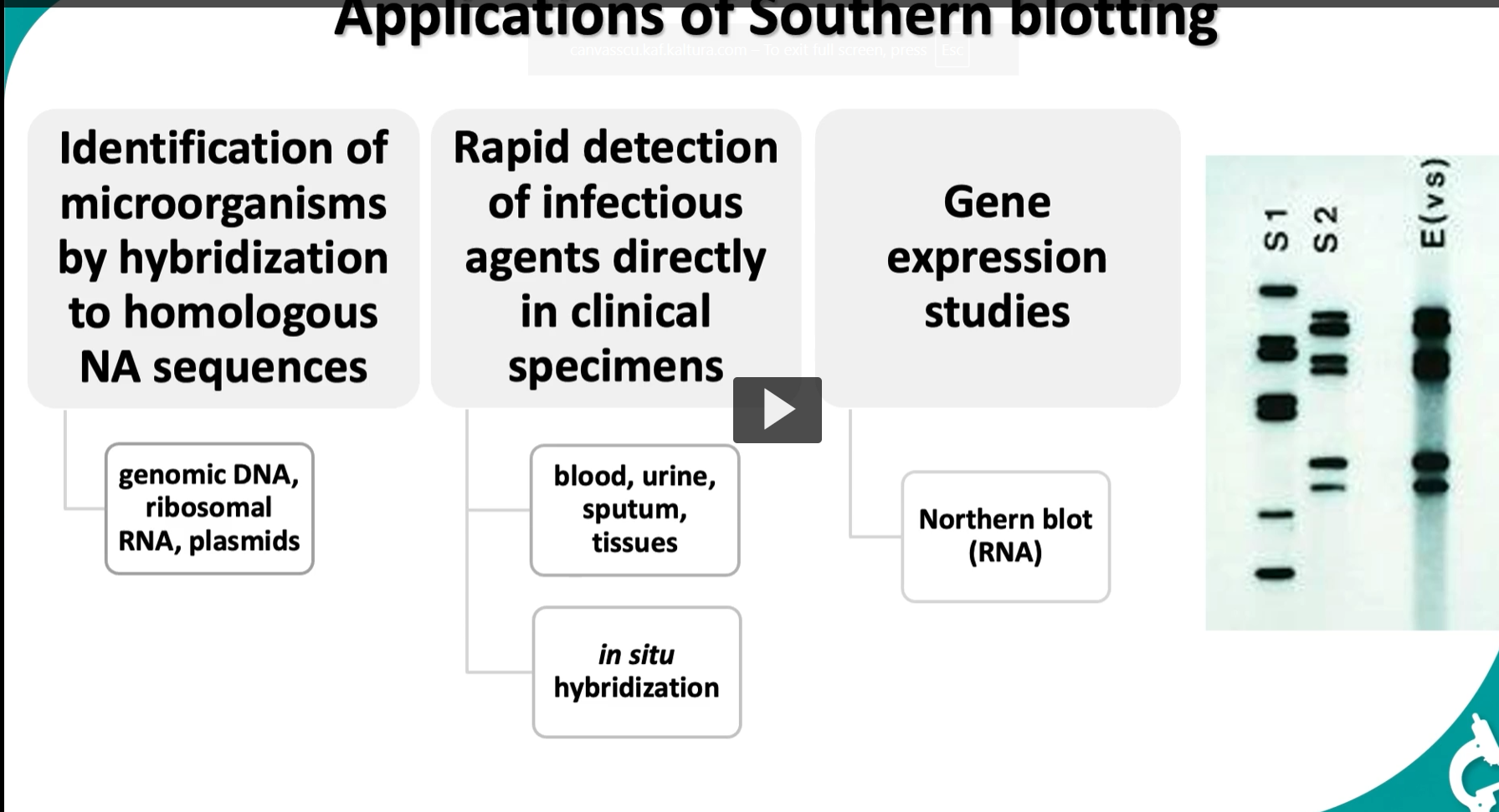
Applications of Southern blotting

---

South blotting allows Identification of microorganisms by hybridization to homologous NA sequences

• genomic DNA, ribosomal RNA, plasmids

---

Southern blotting allows Rapid detection of infectious agents directly in clinical specimens

• blood, urine, sputum, tissues

• in situ hybridization

---

Southern blotting allows Gene expression studies

• Northern blot (RNA)

Different HPV subtypes have different cancer risks, and molecular probes can detect which subtype is present.

👉 This lets us:

• diagnose infection

• predict cancer risk

---

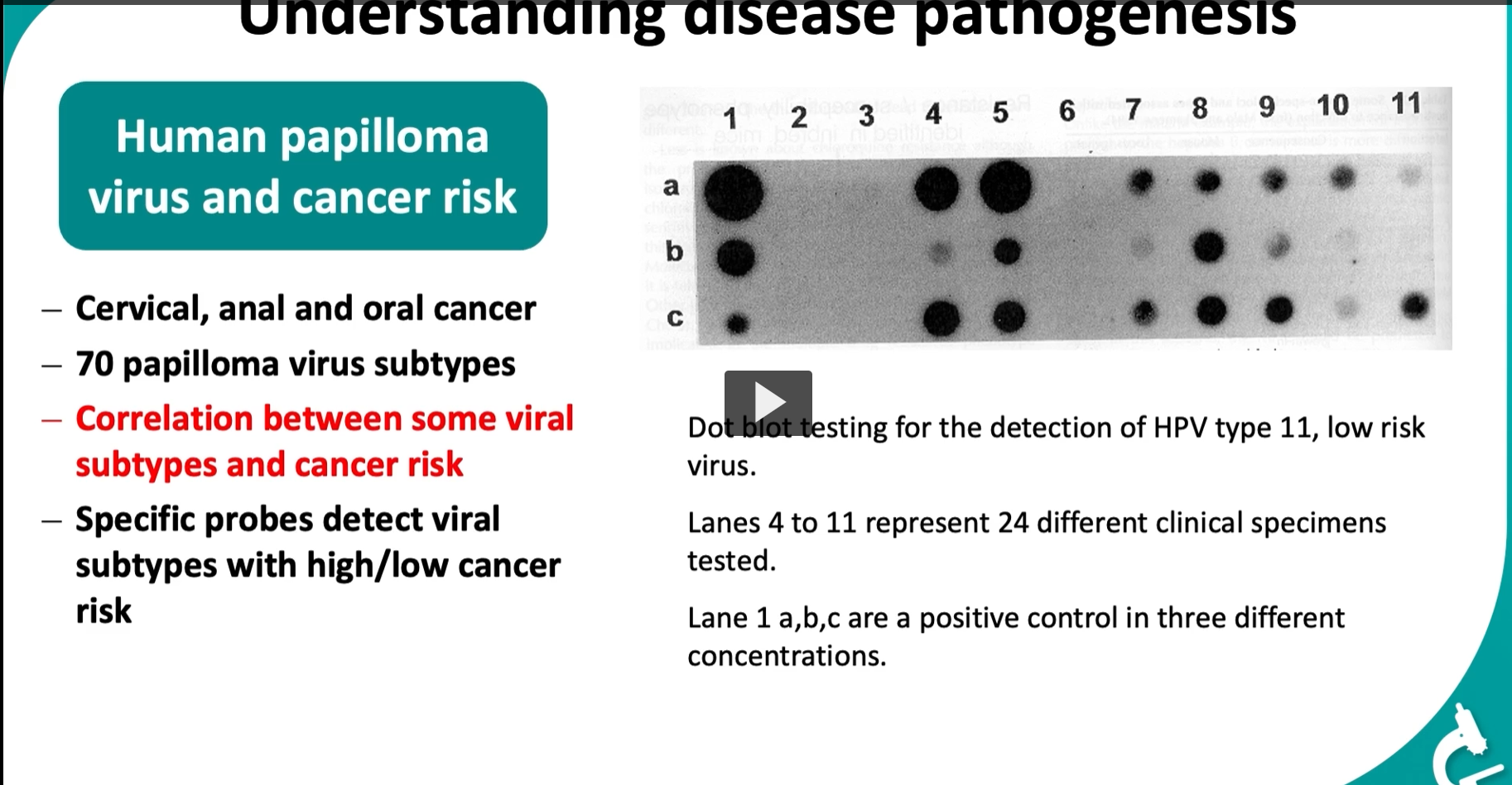
🦠 Part 1: HPV and cancer What is HPV?

• Human papillomavirus (HPV) = a DNA virus

• Infects epithelial cells (skin, mucosa)

---

Diseases associated:

• Cervical cancer

• Anal cancer

• Oral (oropharyngeal) cancer

---

Key concept:

• There are ~70+ HPV subtypes

• NOT all are dangerous

👉 Two categories:

• Low-risk types (e.g., HPV 6, 11) → warts

• High-risk types (e.g., HPV 16, 18) → cancer

---

🔴 Critical point on the slide

“Correlation between some viral subtypes and cancer risk”

👉 Meaning:

• The specific DNA sequence (genotype) determines how dangerous the virus is

---

🧪 Part 2: How we detect this (dot blot)

This slide shows a dot blot (a simpler version of Southern blot).

---

🔬 What is a dot blot?

• DNA samples are placed as dots on a membrane

• No size separation (unlike gel electrophoresis)

• A probe is added

👉 If the target HPV DNA is present → dot becomes dark

---

📊 Interpreting the image Layout:

• Columns labeled 1–11 = different samples

• Rows a, b, c = different concentrations (controls)

---

Controls (Lane 1):

• a, b, c = positive control

• Show strong signals at different concentrations

👉 Confirms:

The test is working properly

---

Clinical samples (Lanes 4–11):

• Each dot = one patient/sample

👉 Dark dot → HPV DNA present
👉 No dot → HPV not detected

---

Important detail:

• This test is specifically detecting:

  HPV type 11 (low-risk virus)

So:

• Positive result → patient has low-risk HPV

• Negative → no HPV 11 detected (could still have other types!)

---

🧠 Why probes matter

“Specific probes detect viral subtypes”

• Each probe is designed for a specific HPV DNA sequence

• You can:

  • distinguish HPV 11 vs HPV 16

  • classify low vs high cancer risk

---

🔥 Clinical significance

This is HUGE in medicine:

• Determines:

  • Who is at risk for cancer

  • Who needs closer monitoring

• Used in:

  • Pap smear follow-ups

  • HPV screening

---

🧩 High-yield summary

Molecular hybridization techniques (like dot blot) use sequence-specific probes to detect HPV subtypes, allowing identification of infections and assessment of cancer risk based on viral genotype.

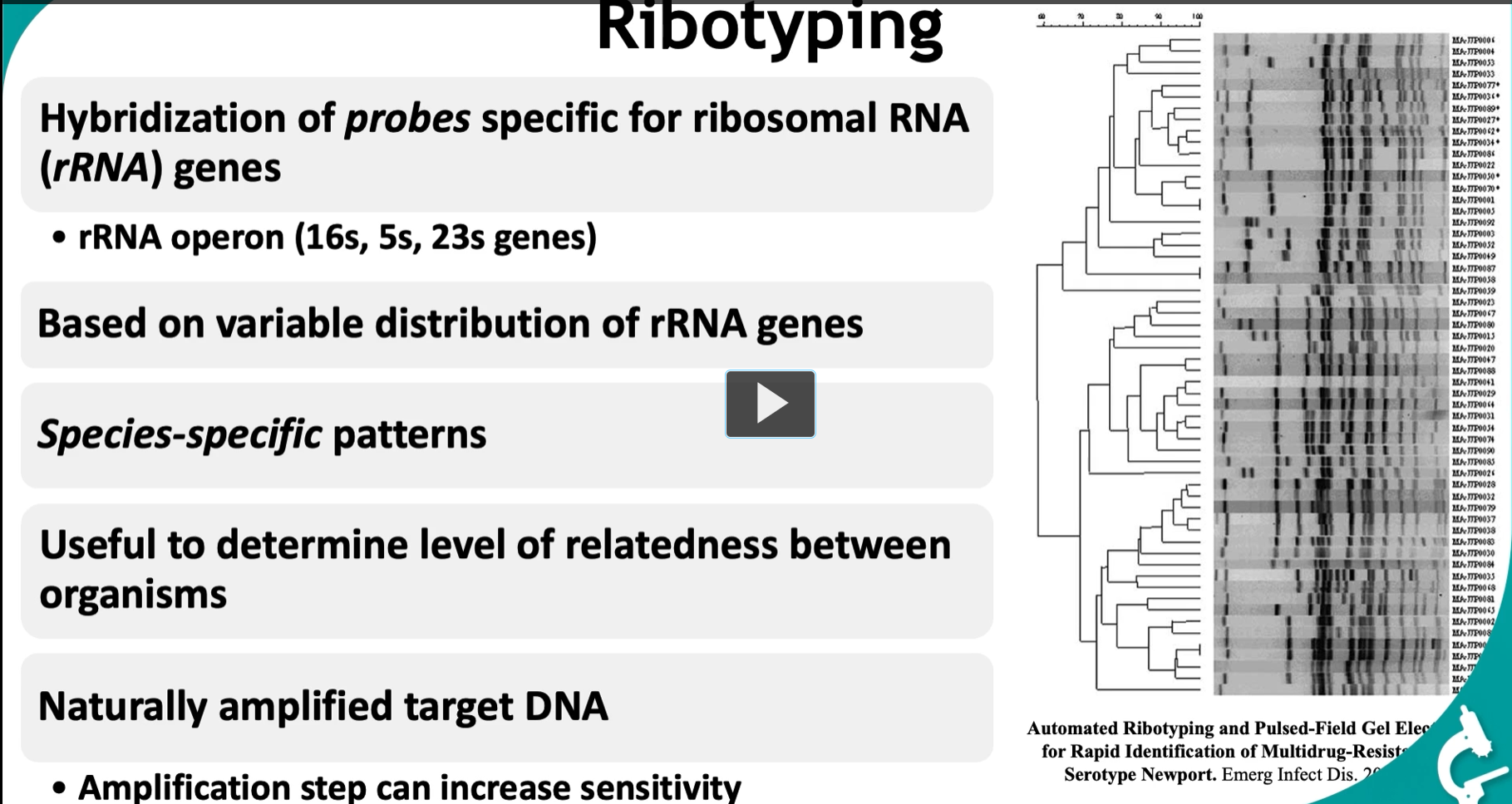
This slide is about ribotyping, a molecular method used to identify and compare bacteria based on their rRNA genes. Here’s the logic step-by-step:

---

🧬 Big Idea

Ribotyping = using rRNA gene patterns as a “genetic fingerprint” to identify and compare organisms.

---

🧪 What are rRNA genes?

Bacteria have ribosomal RNA (rRNA) genes, which are essential for making ribosomes.

These include:

• 16S rRNA

• 23S rRNA

• 5S rRNA

👉 Together they form the rRNA operon

---

🔑 Why rRNA genes are special

• Highly conserved → similar across many bacteria

• BUT also have variable regions → allow differentiation

👉 This balance makes them perfect for:

identification + evolutionary comparison

---

🔬 How ribotyping works 1. DNA is cut (restriction enzymes)

• Break genome into fragments

---

2. Fragments separated (gel electrophoresis)

• Different sizes spread out

---

3. Probe hybridization

• Use probes that bind specifically to rRNA genes

👉 Only fragments containing rRNA genes will be detected

---

4. Band pattern is generated

• This pattern = ribotype

---

🧬 Key concept: “variable distribution”

Different bacteria have rRNA genes in different locations and numbers

So after cutting DNA:

• rRNA-containing fragments differ in size and position

👉 Result:

• Each species → unique banding pattern

---

📊 Species-specific patterns

• Same species → similar pattern

• Different species → different pattern

👉 This is like a:

barcode for bacterial identity

---

🌳 Determining relatedness

The tree (dendrogram on right side):

• Groups organisms based on similarity of patterns

• Closer branches → more closely related

👉 Used for:

• taxonomy

• evolutionary relationships

• outbreak tracking

---

🔥 “Naturally amplified target DNA”

This is VERY important:

• rRNA genes exist in multiple copies per genome

👉 Meaning:

• Easier to detect

• Stronger signal

---

Amplification (optional)

• PCR can further increase sensitivity

• Useful for low DNA samples

---

🧠 Why ribotyping is useful

• Identify unknown bacteria

• Compare strains

• Study evolution

• Track infections

---

🧩 High-yield summary

Ribotyping uses probes targeting rRNA genes to generate species-specific banding patterns, allowing identification and determination of genetic relatedness among organisms.

---

🧠 Simple mental model

• rRNA genes = “landmarks” in the genome

• Restriction enzymes = “cutting map”

• Pattern = “genetic fingerprint”

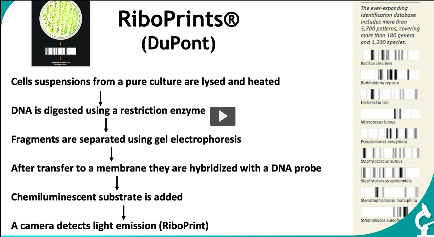
This slide is showing RiboPrints®, which is basically an automated, standardized version of ribotyping used for bacterial identification.

---

🧬 Big Idea

RiboPrint = generate a DNA “barcode” (fingerprint) using rRNA genes and match it to a database to identify the organism.

👉 Think:
“Cut DNA → detect rRNA fragments → create pattern → match to database.”

---

🔬 Step-by-step (what’s happening) 1. Cells from a pure culture are lysed

• Break open bacteria to release DNA

👉 “Pure culture” = only one organism present
→ important for accurate identification

---

2. DNA digestion (restriction enzyme)

• DNA is cut at specific sequences

👉 Result:

• Many fragments of different sizes

---

3. Gel electrophoresis

• Fragments are separated by size

👉 Creates a band pattern

---

4. Transfer + hybridization (like Southern blot)

• DNA is transferred to a membrane

• A probe for rRNA genes is added

👉 Only fragments containing rRNA genes are detected

---

5. Chemiluminescent detection

• A substrate is added

• Bound probes produce light

👉 No color bands—this is detected as light emission

---

6. Camera detection → RiboPrint

• A camera records the pattern

• This pattern = RiboPrint (DNA fingerprint)

---

📊 What happens next (most important part)

The system compares your pattern to a large database

From the slide:

• 5,700+ patterns

• 180+ genera

• 1,200+ species

👉 Match = organism identified

---

🧠 Why rRNA genes are used

• Present in all bacteria

• Have:

  • conserved regions → probe can bind

  • variable distribution → different patterns

👉 Perfect for identification

---

📌 Right-side examples (what you’re seeing)

Different banding patterns correspond to different species:

• Escherichia coli

• Staphylococcus aureus

• Pseudomonas aeruginosa

• etc.

👉 Each species = unique barcode pattern

---

🔥 Why this is useful

• Fast identification of bacteria

• Standardized (automated system)

• Useful in:

  • clinical microbiology

  • food safety

  • outbreak investigations

---

🧩 High-yield summary

RiboPrint is an automated ribotyping method that generates rRNA-based DNA fingerprints and compares them to a database to identify bacterial species.

---

🧠 Simple mental model

• Restriction enzyme = scissors

• rRNA probe = target detector

• Pattern = barcode

• Database = scanner system (like a grocery store)

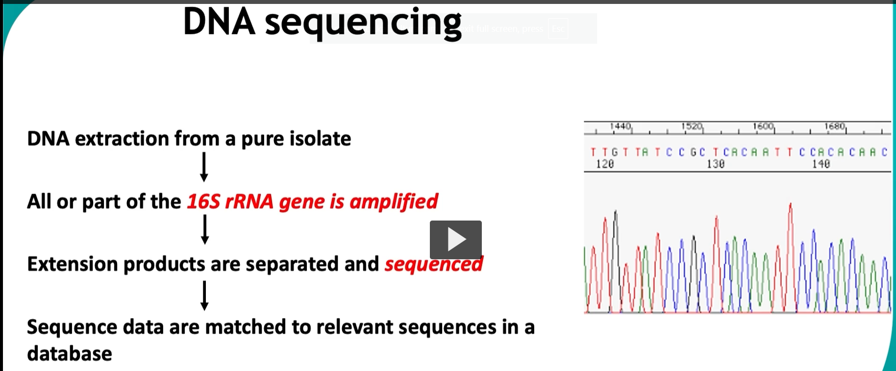
This slide is showing how DNA sequencing (specifically 16S rRNA sequencing) is used to identify bacteria—this is the modern gold standard replacing many older methods like ribotyping.

---

🧬 Big Idea

Sequence the 16S rRNA gene → compare to a database → identify the organism.

👉 Think:
“Read the DNA code → match it like a fingerprint.”

---

🔬 Step-by-step explanation 1. DNA extraction from a pure isolate

• Take a single bacterial species (pure culture)

• Extract its DNA

👉 Important:

Pure isolate = ensures you’re sequencing ONE organism

---

2. Amplify the 16S rRNA gene (PCR)

• Use PCR to copy the 16S rRNA gene

👉 Why 16S?

• Present in all bacteria

• Has:

  • conserved regions → primers can bind

  • variable regions → distinguish species

👉 This is the KEY:

Same gene in all bacteria, but slightly different sequence

---

3. Extension products are separated and sequenced

• DNA is sequenced (often via Sanger sequencing)

👉 The graph on the right = chromatogram

• Each peak = a nucleotide:

  • A, T, C, G (different colors)

👉 Output:

• A string like: ATCGTTACG…

---

4. Match sequence to database

• Compare your sequence to:

  • GenBank

  • BLAST

  • clinical databases

👉 Result:

• Closest match = organism identity

---

🧠 Why this works (core concept)

The 16S rRNA gene is like a biological barcode.

• Conserved → universal detection

• Variable → species-level identification

---

🔥 Why this is powerful

Compared to older methods:

Method	What it uses	Limitation
ELISA	proteins	indirect
PFGE	patterns	complex
Ribotyping	band patterns	lower resolution
Sequencing	actual DNA sequence	most precise

---

🧪 Clinical significance

Used for:

• Identifying unknown bacteria

• Detecting rare or unculturable organisms

• Diagnosing infections

• Microbiome studies

---

🧩 High-yield summary

16S rRNA sequencing identifies bacteria by amplifying and sequencing a conserved gene with variable regions and matching it to known sequences in databases.

---

🧠 Simple mental model

• PCR = photocopier

• Sequencing = reading the letters

• Database = search engine

• Match = organism ID

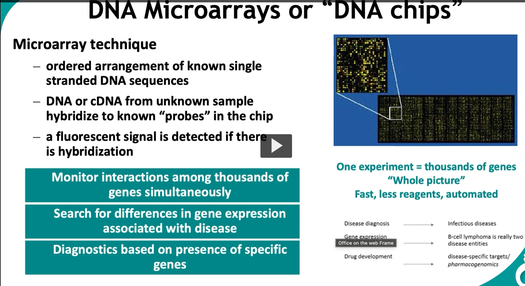
This slide is about DNA microarrays (“DNA chips”), which let you analyze thousands of genes at once. It’s a big step up from single-gene methods.

---

🧬 Big Idea

Microarrays = test many genes simultaneously by hybridization to known DNA probes on a chip.

👉 Think:
“Thousands of probes on a chip → your sample binds → glowing pattern tells the story.”

---

🔬 How the microarray works (step-by-step) 1. Chip contains known DNA probes

• The chip has thousands of spots

• Each spot = a known single-stranded DNA sequence (a gene or part of a gene)

👉 Like:

A grid of “questions” (each probe asks: is this gene present or expressed?)

---

2. Sample DNA or cDNA is added

• From an unknown sample:

  • DNA → for gene presence

  • cDNA → for gene expression (most important use)

👉 cDNA is made from mRNA → reflects which genes are active

---

3. Hybridization occurs

• If your sample contains a matching sequence → it binds (hybridizes) to that spot

👉 Specific binding = sequence match

---

4. Fluorescent signal detection

• Sample is labeled with a fluorescent dye

• Where binding occurs → spot glows

👉 Brightness = amount of gene expression (or abundance)

---

📊 What you get (the image on right)

• A grid of colored dots:

  • Bright = high expression

  • Dim = low expression

  • No signal = not expressed

👉 This gives a global snapshot of gene activity

---

🧠 What makes this powerful 🔹 “One experiment = thousands of genes”

• Instead of testing 1 gene → test entire genome patterns

---

🔹 “Whole picture”

• You see how genes interact

• Not just “on/off” → but patterns

---

🔬 Applications (from slide) 1. Gene expression analysis

• Compare:

  • healthy vs diseased tissue

• Example:

  • cancer vs normal cells

👉 Can reveal:

Which genes are turned ON or OFF in disease

---

2. Disease diagnosis

• Detect:

  • infectious agents

  • genetic signatures

---

3. Cancer classification

• Example from slide:

  • B-cell lymphoma → actually two different diseases based on gene expression

👉 Same appearance, different molecular behavior

---

4. Drug development

• Identify:

  • disease-specific pathways

  • drug targets

• Pharmacogenomics:

  • how patients respond differently to drugs

---

🧩 Key conceptual connection

Microarrays don’t just tell you what is there → they tell you what is active.

---

🔥 High-yield summary

DNA microarrays use thousands of immobilized DNA probes to detect gene presence or expression via fluorescent hybridization, enabling large-scale analysis of gene activity in a single experiment.

---

🧠 Simple mental model

• Chip = thousands of locks

• Sample DNA = keys

• Binding = correct key fits lock

• Fluorescence = light turns on when match happens

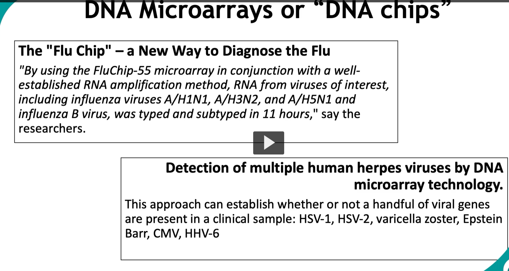
DNA Microarrays or “DNA chips”

---

The “Flu Chip” – a New Way to Diagnose the Flu

“By using the FluChip-55 microarray in conjunction with a well-established RNA amplification method, RNA from viruses of interest, including influenza viruses A/H1N1, A/H3N2, and A/H5N1 and influenza B virus, was typed and subtyped in 11 hours,” say the researchers.

---

Detection of multiple human herpes viruses by DNA microarray technology.

This approach can establish whether or not a handful of viral genes are present in a clinical sample: HSV-1, HSV-2, varicella zoster, Epstein Barr, CMV, HHV-6

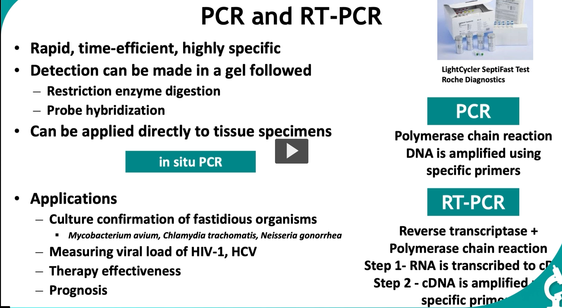
This slide is one of the most important in molecular diagnostics—it explains PCR and RT-PCR, which are the backbone of modern testing (COVID tests, HIV viral load, etc.).

---

🧬 Big Idea

PCR = make millions of copies of a specific DNA sequence.
RT-PCR = convert RNA → DNA → then amplify it.

👉 Think:
“Find a tiny piece of genetic material → copy it → detect it.”

---

🔬 PART 1: PCR (Polymerase Chain Reaction) 🧪 What PCR does

• Takes a small amount of DNA

• Uses specific primers to target a sequence

• Amplifies it → millions of copies

---

⚙ How it works (conceptually)

PCR cycles repeat:

1. Denaturation → DNA strands separate

2. Annealing → primers bind to target sequence

3. Extension → DNA polymerase copies DNA

👉 Repeat ~30 cycles → exponential amplification

---

🔑 Key feature:

Highly specific (because primers define the target)

---

🧪 Detection (from slide)

After PCR:

• Run on gel electrophoresis

• Or:

  • restriction enzyme digestion

  • probe hybridization

👉 Confirms identity of amplified DNA

---

🧬 PART 2: RT-PCR (for RNA)

Used when the target is RNA, not DNA

---

⚙ Steps: Step 1: Reverse transcription

• Reverse transcriptase enzyme

• Converts RNA → cDNA

Step 2: PCR

• Amplify the cDNA using primers

---

🔑 Key idea:

RNA cannot be amplified directly → must first become DNA

---

🧪 “In situ PCR”

• PCR done directly in tissue

• Preserves location of DNA/RNA

👉 Shows:

• where the pathogen or gene is inside tissue

---

⚡ Why PCR is powerful

• Rapid → results in hours

• Highly sensitive → detects tiny amounts

• Highly specific → sequence-targeted

---

🧠 Applications (from slide) 1. Detect hard-to-grow organisms

• Mycobacterium avium

• Chlamydia trachomatis

• Neisseria gonorrhea

👉 Important because:

Some bacteria are slow or difficult to culture

---

2. Measure viral load

• HIV-1

• HCV

👉 Quantifies:

How much virus is in the body

---

3. Monitor therapy

• Is treatment working?

• Viral load decreasing?

---

4. Prognosis

• High viral load → worse outcome

• Low viral load → better prognosis

---

🧪 Real-world example (on slide)

LightCycler SeptiFast Test (Roche)

• Detects pathogens directly from blood

• Used in sepsis diagnosis

---

🔥 High-yield summary

PCR amplifies specific DNA sequences using primers, while RT-PCR first converts RNA to cDNA before amplification, enabling rapid, sensitive detection and quantification of pathogens.

---

🧠 Simple mental model

• PCR = DNA photocopier

• RT-PCR = translate RNA → then copy it

• Primers = address labels telling copier what to copy

---

⚠ Exam tip (very important)

• PCR = DNA detection

• RT-PCR = RNA detection (viruses like HIV, COVID)

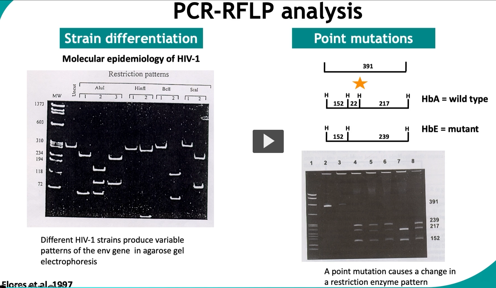
This slide is about PCR-RFLP, a classic method used to detect genetic differences (mutations or strain variation) by combining PCR with restriction enzymes.

---

🧬 Big Idea

PCR-RFLP = amplify DNA → cut with restriction enzymes → analyze fragment pattern.

👉 If the DNA sequence changes → the cutting pattern changes → the band pattern changes.

---

🔬 Step-by-step (core workflow) 1. PCR amplification

• Target a specific gene (e.g., HIV env gene, hemoglobin gene)

• Make many copies

---

2. Restriction enzyme digestion

• Add a restriction enzyme (e.g., AluI, HinfI)

• Enzyme cuts DNA at specific sequences

👉 Important:

If a mutation changes the sequence → enzyme may cut differently or not at all

---

3. Gel electrophoresis

• Separate fragments by size

• Visualize band pattern

---

🧠 Key principle

DNA sequence → determines restriction sites → determines band pattern

---

🧪 LEFT SIDE: Strain differentiation (HIV example) What’s happening:

• Different HIV-1 strains have slightly different DNA sequences

• When cut with enzymes → produce different fragment sizes

👉 Result:

• Each strain → unique banding pattern

---

Why useful:

• Track infection spread

• Identify sources of outbreaks

• Compare viral strains

👉 This is molecular epidemiology

---

🧬 RIGHT SIDE: Point mutation example (HbA vs HbE)

This is the most important concept.

---

🧪 Wild type (HbA)

• Normal DNA sequence

• Restriction enzyme recognizes its site → cuts

👉 Produces:

• Multiple fragments (e.g., 152, 22, 217)

---

🧪 Mutant (HbE)

• Single base change (point mutation)

• Alters restriction site

👉 Result:

• Enzyme can’t cut at that site anymore

• Fragment sizes change (e.g., 152, 239)

---

📊 Gel interpretation

• Different band sizes = different DNA sequence

• Compare lanes:

  • Same pattern → same genotype

  • Different pattern → mutation present

---

🔥 Key concept (HIGH-YIELD)

A single nucleotide change can:

• create a new restriction site

• destroy an existing one

👉 → changes band pattern

---

🧠 Why this works

Restriction enzymes are:

• sequence-specific “molecular scissors”

So even:

1 base change = different cutting = different pattern

---

🧩 High-yield summary

PCR-RFLP detects genetic variation by amplifying DNA, digesting it with restriction enzymes, and identifying sequence differences based on fragment size patterns.

---

🧠 Simple mental model

• PCR = copy the sentence

• Restriction enzyme = cut at specific words

• Mutation = changes the word → cut changes

• Gel = shows where cuts happened

---

⚠ Exam tip

• Used for:

  • mutation detection

  • strain typing

• Being replaced by:

  • sequencing (more precise)

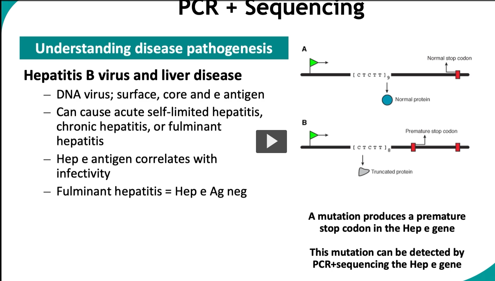
This slide shows how PCR + sequencing helps us understand disease mechanisms (pathogenesis)—using Hepatitis B virus (HBV) as the example.

---

🧬 Big Idea

A specific mutation in HBV changes a viral protein → changes disease behavior → detected by PCR + sequencing.

👉 This connects:
genetic mutation → protein change → clinical outcome

---

🦠 Part 1: Hepatitis B basics

• HBV is a DNA virus

• Produces key antigens:

  • Surface antigen (HBsAg)

  • Core antigen (HBcAg)

  • e antigen (HBeAg)

---

🔑 Important concept:

HBeAg = marker of infectivity

• If HBeAg is present → high viral replication / high infectivity

• If absent → usually lower infectivity… BUT not always (important!)

---

⚠ Disease outcomes

HBV infection can cause:

• Acute hepatitis (self-limited)

• Chronic hepatitis

• Fulminant hepatitis (severe, rapid liver failure)

---

🧬 Part 2: The mutation (right side diagram) Normal case (A)

• Gene has a normal stop codon at the correct position

• Full protein is made → functional HBeAg

👉 Result:

• Virus produces HBeAg

• Infection is detectable via this marker

---

Mutant case (B)

• A point mutation introduces a premature stop codon

👉 What happens:

• Protein production stops early

• Truncated (shortened) protein is made

• HBeAg is NOT produced

---

🔥 Critical clinical insight

Fulminant hepatitis = HBeAg negative

BUT:

• Virus is still active

• Just not producing detectable HBeAg

👉 This can be misleading clinically

---

🧠 Why this matters

• Patient appears:

  • HBeAg negative

• But actually:

  • Still highly infected and dangerous

👉 This mutation explains:

Why some severe HBV cases lack HBeAg

---

🧪 How we detect this (PCR + sequencing) Step 1: PCR

• Amplify the HBe gene

---

Step 2: Sequencing

• Read the DNA sequence

• Identify:

  • mutation causing premature stop codon

---

Result:

• Detect hidden mutant virus

---

🧩 Conceptual connection

Level	What happens
DNA	mutation (point mutation)
Protein	truncated HBeAg
Lab test	HBeAg negative
Clinical effect	severe disease (fulminant hepatitis)

---

🔥 High-yield summary

A mutation in the HBV Hep e gene creates a premature stop codon, preventing HBeAg production and leading to severe disease; this mutation can be detected by PCR and DNA sequencing.

---

🧠 Simple mental model

• Normal gene → full protein → detectable marker

• Mutated gene → early stop → no marker → hidden but dangerous infection

---

⚠ Exam tip (VERY important)

HBeAg negative does NOT always mean low infectivity
→ Could be a pre-core mutant HBV

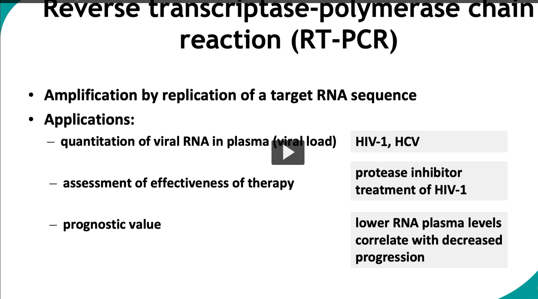
This slide focuses specifically on RT-PCR for RNA viruses, especially how it’s used clinically to measure viral load and monitor disease.

---

🧬 Big Idea

RT-PCR measures how much viral RNA is present in a patient → tells you how active the infection is.

👉 Think:
“More RNA = more virus = worse disease (usually)”

---

🔬 What RT-PCR is doing (core concept) Step 1: Reverse transcription

• Viral RNA → converted into cDNA using reverse transcriptase

Step 2: PCR amplification

• cDNA is amplified → millions of copies

👉 Result:

• Even tiny amounts of virus can be detected and quantified

---

📊 What makes this slide important: QUANTITATION

Unlike regular PCR:

RT-PCR can measure how much virus is present (viral load)

---

🧪 Application 1: Viral load measurement Used for:

• HIV-1

• Hepatitis C (HCV)

👉 Sample:

• Blood plasma

---

What is “viral load”?

The amount of viral RNA in the blood

• High viral load → lots of virus

• Low viral load → less virus

---

💊 Application 2: Monitoring therapy

Example from slide:

• Protease inhibitor treatment (HIV)

👉 After treatment:

• Viral replication is blocked

• RT-PCR shows decreasing RNA levels

---

Key concept:

RT-PCR = real-time feedback on treatment effectiveness

---

📉 Application 3: Prognostic value

Viral load predicts disease progression

From slide:

• Lower RNA plasma levels → decreased progression

👉 Meaning:

• Lower viral load → better outcome

• Higher viral load → worse prognosis

---

🧠 Clinical interpretation

Viral Load	Meaning
High	Active infection, poor control
Decreasing	Treatment working
Undetectable	Virus suppressed

---

🔥 Why RT-PCR is so powerful

• Extremely sensitive

• Quantitative (not just yes/no)

• Works for RNA viruses

---

🧩 High-yield summary

RT-PCR converts viral RNA to cDNA and amplifies it to quantify viral load, which is used to monitor treatment effectiveness and predict disease progression.

---

🧠 Simple mental model

• RT step = translate RNA → DNA

• PCR = copy it

• Output = how much virus is present

---

⚠ Exam tip (very important)

RT-PCR is the gold standard for viral load monitoring (HIV, HCV)

NOT just detection—quantification

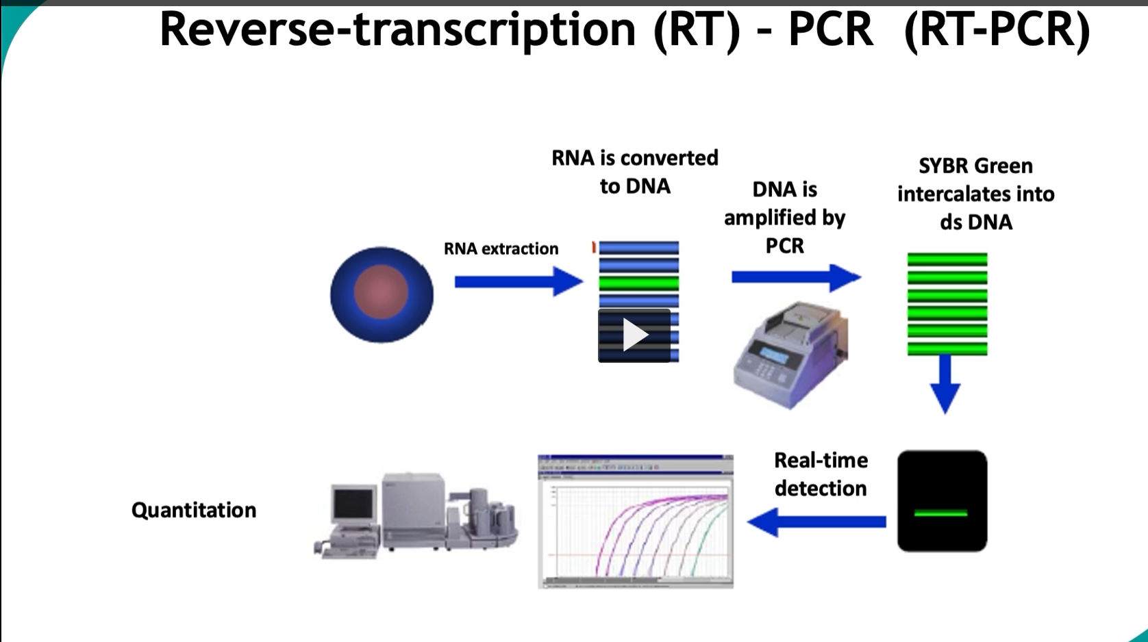
This slide is showing real-time RT-PCR (qRT-PCR)—the most advanced and clinically important version of PCR, used to detect AND quantify RNA in real time.

---

🧬 Big Idea

qRT-PCR = convert RNA → amplify DNA → measure fluorescence in real time → quantify how much RNA was present.

👉 Think:
“Copy it AND measure it while it’s happening.”

---

🔬 Step-by-step (what’s happening in the diagram)

---

1. RNA extraction

• Start with a sample (blood, tissue, swab)

• Extract RNA (e.g., viral RNA like HIV, SARS-CoV-2)

---

2. RNA → DNA (Reverse transcription)

• Enzyme: reverse transcriptase

• Converts RNA → cDNA

👉 Required because:

PCR only works on DNA

---

3. DNA amplification (PCR)

• cDNA is amplified through cycles

• Each cycle → doubles DNA amount

---

4. SYBR Green binds DNA

• SYBR Green dye intercalates into double-stranded DNA

• When bound → fluoresces (glows)

👉 More DNA → more fluorescence

---

5. Real-time detection

• Machine measures fluorescence after each cycle

👉 Unlike regular PCR:

• You don’t wait until the end

• You monitor amplification live

---

6. Quantitation (most important)

The graph shows curves:

• X-axis = cycle number

• Y-axis = fluorescence

---

📊 Ct value (CRITICAL concept)

Ct (cycle threshold) = cycle at which fluorescence becomes detectable

---

Interpretation:

Ct Value	Meaning
Low Ct (e.g., 15–20)	High starting RNA (lots of virus)
High Ct (e.g., 30–40)	Low starting RNA
No Ct	No detectable RNA

---

🧠 Why this is powerful

• Detects RNA viruses

• Quantifies viral load

• Extremely sensitive

• Extremely fast

---

🧪 Clinical uses

• HIV viral load

• Hepatitis C monitoring

• COVID-19 testing

• Gene expression studies

---

🔥 Key difference from regular PCR

Regular PCR	qRT-PCR
End-point detection	Real-time detection
Qualitative (yes/no)	Quantitative
Gel needed	No gel needed

---

🧩 High-yield summary

Real-time RT-PCR converts RNA to cDNA, amplifies it, and uses fluorescent dyes like SYBR Green to measure DNA accumulation during each cycle, allowing quantification of the original RNA.

---

🧠 Simple mental model

• Reverse transcription = translate RNA → DNA

• PCR = copy it repeatedly

• SYBR Green = glow when DNA increases

• Machine = tracks glow over time

---

⚠ Exam tip

Lower Ct = higher viral load

This is one of the most tested concepts.

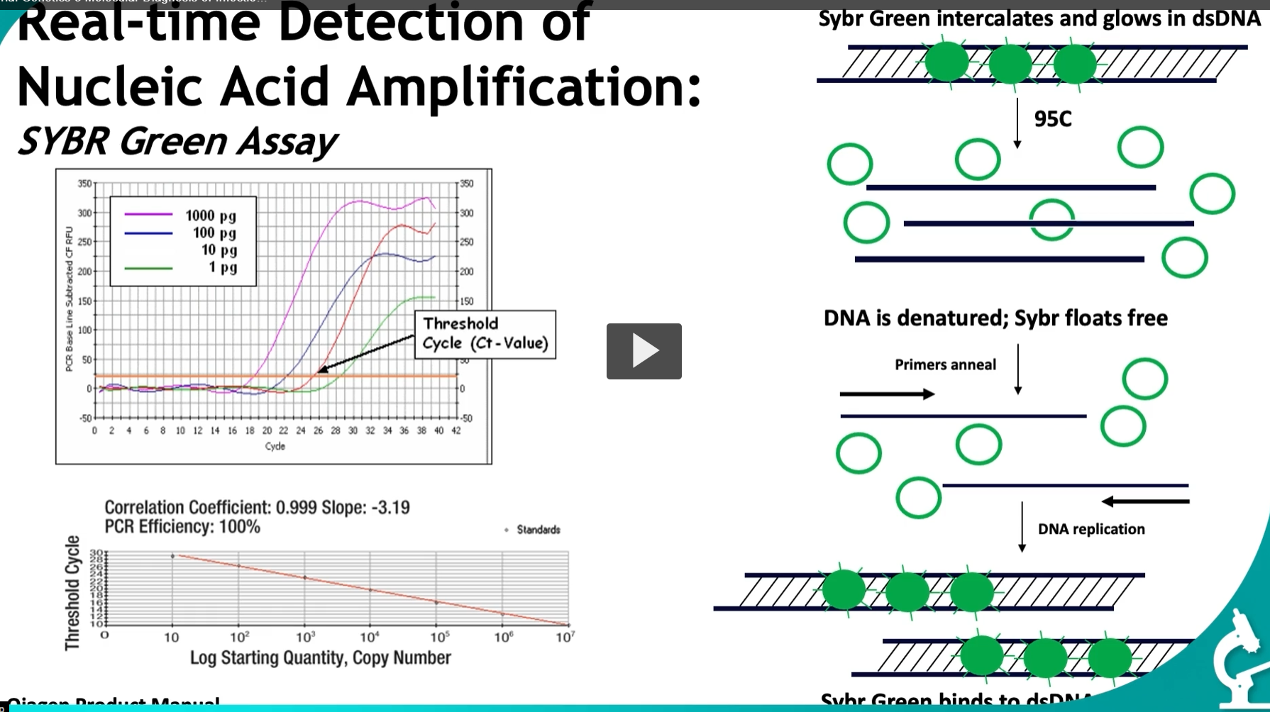
This slide explains how real-time PCR (qPCR) works using SYBR Green and how we quantify DNA using Ct values. This is a very high-yield concept.

---

🧬 Big Idea

SYBR Green glows when bound to double-stranded DNA → more DNA = more fluorescence → measure it each cycle to quantify starting material.

---

🔬 PART 1: What SYBR Green does 🧪 Key property:

• SYBR Green binds (intercalates) into double-stranded DNA (dsDNA)

• When bound → fluoresces (glows)

• When not bound → no signal

---

🔁 What happens during each PCR cycle 🔥 1. Denaturation (95°C)

• DNA strands separate → single-stranded DNA

• SYBR Green falls off

👉 Result:

• Low fluorescence

---

🧬 2. Annealing

• Primers bind to DNA

---

⚙ 3. Extension (replication)

• DNA polymerase makes new strands → dsDNA forms again

• SYBR Green binds again

👉 Result:

• Fluorescence increases

---

🔁 Each cycle:

• More DNA → more SYBR binding → more fluorescence

---

📊 PART 2: The amplification curve

The graph shows:

• X-axis = cycle number

• Y-axis = fluorescence

Each line = different starting amount:

• 1000 pg → highest

• 1 pg → lowest

---

🧠 Key observation

More starting DNA → curve rises earlier

---

📍 Ct value (MOST IMPORTANT)

Ct (threshold cycle) = cycle where fluorescence crosses a set threshold

---

Interpretation:

Starting DNA	Ct value
High (1000 pg)	Low Ct (early detection)
Low (1 pg)	High Ct (late detection)

👉 Inverse relationship:

Ct ↓ = more starting DNA
Ct ↑ = less starting DNA

---

📈 PART 3: Standard curve (bottom graph)

• X-axis = log starting quantity

• Y-axis = Ct

👉 Straight line relationship:

• Used to calculate unknown samples

---

Values on slide:

• Correlation coefficient: 0.999 → very accurate

• Slope: -3.19 → ideal PCR efficiency

• PCR efficiency: ~100%

👉 Meaning:

DNA is doubling perfectly each cycle

---

🧠 Why this matters

This allows:

• Quantification of DNA/RNA

• Viral load measurement

• Gene expression analysis

---

🔥 High-yield summary

SYBR Green qPCR detects DNA amplification in real time by fluorescing when bound to double-stranded DNA, and Ct values are used to determine the initial amount of nucleic acid.

---

🧠 Simple mental model

• DNA doubles → fluorescence doubles

• Machine tracks glow → determines how much you started with

---

⚠ Important limitation (exam tip)

• SYBR Green binds ANY dsDNA
  → includes non-specific products
  → less specific than probe-based methods

---

Ultimate takeaway

The earlier the signal appears (lower Ct), the more target DNA was present initially.

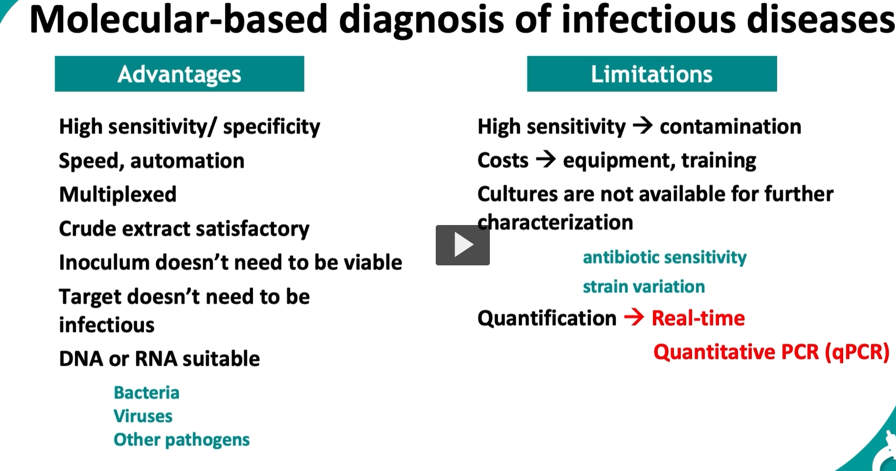
Molecular diagnosis = detecting DNA or RNA of a pathogen directly (instead of growing it in culture).

---

✅ Advantages (Why it’s so good)1. High sensitivity / specificity

• Sensitivity → detects very small amounts of pathogen DNA/RNA

• Specificity → primers/probes bind only to the exact organism

👉 You can detect infections early, even when pathogen levels are low.

---

2. Fast + automated

• PCR results can come in hours (not days)

• Machines run automatically

👉 Huge advantage over culture (which can take days–weeks)

---

3. Multiplexed

• Can test multiple pathogens in one reaction

👉 Example: one test detects flu, RSV, COVID simultaneously

---

4. Crude extract is enough

• Doesn’t require perfectly purified samples

• Can use blood, saliva, sputum directly

👉 Easier sample prep

---

5. Pathogen doesn’t need to be alive

• Detects DNA/RNA even if organism is dead

👉 Useful when:

• Patient already took antibiotics

• Pathogen is hard to culture

---

6. Target doesn’t need to be infectious

• You’re detecting genetic material, not activity

👉 Good for viruses or latent infections

---

7. Works for many organisms

• Bacteria

• Viruses

• Other pathogens (fungi, parasites)

👉 Very versatile technology

---

❌ Limitations (What’s the catch?)1. High sensitivity → contamination risk

• Even tiny contamination = false positive

👉 Example:

• A single DNA fragment from previous sample → wrong diagnosis

---

2. Expensive

• Requires:

  • Specialized machines

  • Trained personnel

👉 Not always accessible everywhere

---

3. No culture = limited follow-up testing

Since you don’t grow the organism:

• ❌ Cannot easily test antibiotic sensitivity

• ❌ Harder to study strain variation

👉 Culture still needed for:

• Drug susceptibility

• Detailed microbiology

---

4. Quantification requires special methods

• Standard PCR = just yes/no

• To measure amount → need real-time PCR (qPCR)

👉 Important for:

• Viral load (HIV, HCV)

• Monitoring treatment

---

🧠 Key Concept to Remember

👉 Molecular tests answer:
“Is the genetic material present?”

BUT NOT always:
“Is the organism alive or clinically relevant?”

---

🔥 High-Yield Exam Summary

• Pros: fast, sensitive, specific, works on non-viable organisms

• Cons: contamination risk, expensive, no culture info

• qPCR = quantification (viral load)