MM - Chapter 9 + Addendum: Image Compression Standards

JPEG Standard

JPEG is an image compression standard that was developed by the “Joint Photographic Experts Group”. JPEG was formally accepted as an international standard in 1992.

JPEG is a lossy image compression method. It employs a transform coding method using the DCT (Discrete Cosine Transform).

An image is a function of i and j (or conventionally x and y) in the spatial domain. The 2D DCT is used as one step in JPEG in order to yield a frequency response which is a function F(u, v) in the spatial frequency domain, indexed by two integers u and v.

JPEG 3 observations

The effectiveness of the DCT transform coding method in JPEG relies on 3 major observations:

Observation 1: Useful image contents change relatively slowly across the image, i.e., it is unusual for intensity values to vary widely several times in a small area, for example, within an 8×8 image block.

• Much of the information in an image is repeated, hence “spatial redundancy”.

Observation 2: Psychophysical experiments suggest that humans are much less likely to notice loss of very high spatial frequency components than the loss of lower frequency components.

• The spatial redundancy can be reduced by largely reducing the high spatial frequency content

Observation 3: Visual acuity (accuracy in distinguishing closely spaced lines) is much greater for gray (“black and white”) than for color.

• Chroma subsampling (4:2:0) is used in JPEG

Main steps in JPEG image compression (Figuur)

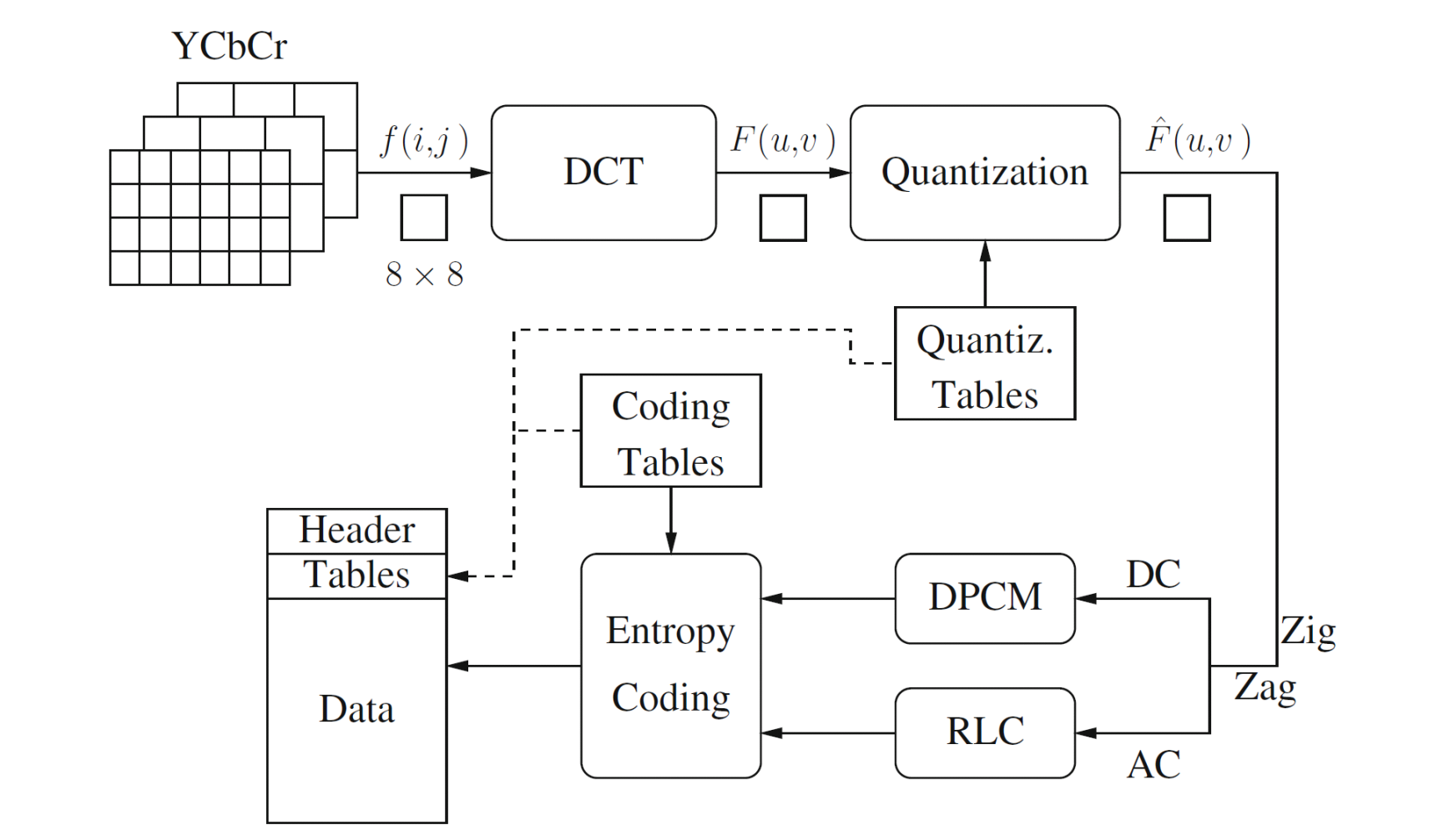
Main steps in JPEG Image Compression

• Transform RGB to YIQ or YUV and subsample color

• DCT on image blocks

• Quantization

• Zig-zag ordering and run-length encoding

• Entropy coding

DCT on image blocks (jpeg)

Each image is divided into 8 × 8 blocks. The 2D DCT is applied to each block image f(i, j), with output being the DCT coefficients F(u, v) for each block.

Using blocks, however, has the effect of isolating each block from its neighboring context. This is why JPEG images look choppy (“blocky”) when a high compression ratio is specified by the user.

jpeg quantization

F(u,v) represents a DCT coefficient, Q(u,v) is a “quantization matrix” entry, and F^(u,v)represents the quantized DCT coefficients which JPEG will use in the succeeding entropy coding.

• The quantization step is the main source for loss in JPEG compression.

• The entries of Q(u, v) tend to have larger values towards the lower right corner. This aims to introduce more loss at the higher spatial frequencies — a practice supported by Observations 1 and 2.

• Default Q(u, v) values obtained from psychophysical studies with the goal of maximizing the compression ratio while minimizing perceptual losses in JPEG images.

Compression control: quantization matrices are scaled based on user-defined quality factor (1-100)

RLC on AC coefficients

RLC aims to turn the F^(u,v) values into sets
{#-zeros-to-skip, next non-zero value}

To make it most likely to hit a long run of zeros: a zig-zag scan is used to turn the 8×8 matrix into a 64-vector.

DPCM on DC Coefficients

The DC coefficients are coded separately from the AC ones.

• using Differential Pulse Code modulation (DPCM)

• (without further quantization, so actually LPC, see Chapter 5)

If the DC coefficients for the first 5 image blocks are 150, 155, 149, 152, 144, then the DPCM would produce 150, 5, -6, 3, -8, assuming di​ = DCi​ − DC_(i-1), and d0​ = DC0​

entropy coding jpeg

• The DC and AC coefficients finally undergo an entropy coding step to gain a possible further compression

• Use DC as an example: each DPCM-coded DC coefficient is represented by (SIZE, AMPLITUDE), where SIZE indicates how many bits are needed for representing the coefficient, and AMPLITUDE contains the actual bits

• In the example we’re using, codes 150, 5, −6, 3, −8 will be turned into

  • (8, 10010110), (3, 101), (3, 001), (2, 11), (4, 0111)

• SIZE is Huffman coded since smaller SIZEs occur much more often. AMPLITUDE is not Huffman coded, its value can change widely so Huffman coding has no appreciable benefit

JPEG Modes (4)

(zie ook volgende vraag)

Sequential Mode

• The default JPEG mode, implicitly assumed in the discussions so far. Each graylevel image or color image component is encoded in a single left-to-right, top-to-bottom scan.

Progressive Mode

• Progressive JPEG delivers low quality versions of the image quickly, followed by higher quality passes.

  1. Spectral selection: Takes advantage of the “spectral” (spatial frequency spectrum) characteristics of the DCT coefficients: higher AC components provide detail information.

     • Scan 1: Encode DC and first few AC components, e.g., AC1, AC2.

     • Scan 2: Encode a few more AC components, e.g., AC3, AC4, AC5.

     • ...

     • Scan k: Encode the last few ACs, e.g., AC61, AC62, AC63.

  2. Successive approximation: Instead of gradually encoding spectral bands, all DCT coefficients are encoded simultaneously but with their most significant bits (MSBs) first.

     • Scan 1: Encode the first few MSBs, e.g., Bits 7, 6, 5, 4.

     • Scan 2: Encode a few more less significant bits, e.g., Bit 3.

     • ...

     • Scan m: Encode the least significant bit (LSB), Bit 0.

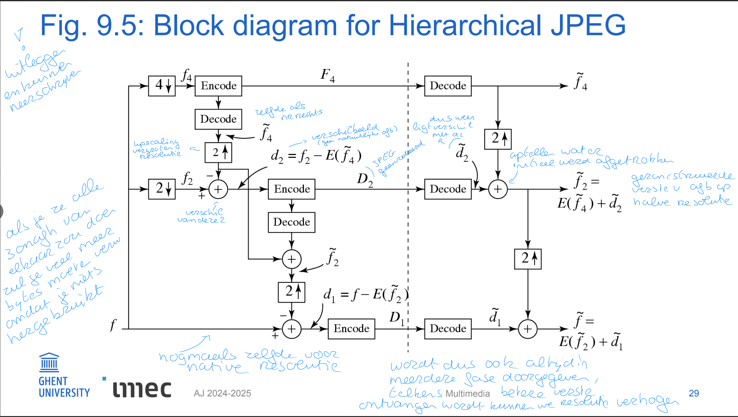
Hierarchical Mode

• The encoded image at the lowest resolution is basically a compressed low-pass filtered image, whereas the images at successively higher resolutions provide additional details (differences from the lower resolution images).

• Similar to Progressive JPEG, the Hierarchical JPEG images can be transmitted in multiple passes progressively improving quality.

Lossless Mode

• discussed in Chapter 6, to be replaced by JPEG-LS

hierarchical mode figuur + uitleg

JPEG-LS standard

• wat

• 3 main steps

• Specifically aimed at lossless encoding

  • not the same as the lossless mode of JPEG (confusing, I know)

• Supports both lossless and near-lossless coding

• Core = low-complexity lossless compression algorithm (LOCO-I)

  • exploits the concept of context modeling (conditional probabilities)

  • three main steps

    • prediction

    • context determination

    • residual coding

LOCO-I three components

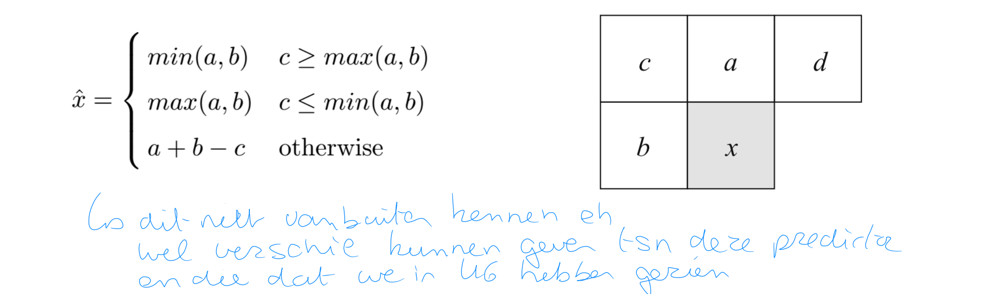
Prediction

• usually, better prediction is achieved when considering image features like edges (but is complex)

• LOCO-I uses a fixed predictor with primitive tests for directionality

  

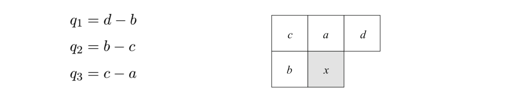
Context Determination

• 3-component context vector Q=(q1 ,q2 ,q3 ) where

• qi are quantized by quantizer with decision boundaries -4,...-1,0,1,...4

• if q1 of Q is negative, we replace Q by –Q

• as such: 365 different context states (stored as an integer)

  

Residual Coding

it can be shown that the error residuals follow a two-sided geometric distribution (TSGD), and they are coded using adaptively selected codes

• based on Golomb codes, which are optimal for geometric distributions

JPEG-LS near lossless mode

• reconstructed samples deviate from the original by no more than δ

• lossless mode is then a special case for which δ = 0

• the residual ε is quantized using a uniform quantizer with step-size 2δ+1:

  

• only a small number of δ values are allowed, the division can be implemented using lookup tables.

• prediction and context determination are based on quantized values

Block based hybrid model for video prediction

Integration of motion estimation into a video compression framework

Hybrid structure of video compression framework, combining

• block-based motion prediction (for temporal correlation)

• block-based transform coding (for spatial correlation)

Basic hybrid structure has been used for a long time

• progressive refinements and enhancements

• double coding performance ca. every 10 years

Prediction modes (forward, backward, bidirectional) lead to different coding types and coding structures

• I-pictures or slices: INTRA coded

• P-pictures or slices: INTER coded, based on 1 reference picture

• B-pictures or slices: INTER coded, based on 1 or 2 reference pictures

• (IDR pictures)

INTRA coding within video codecs became more efficient than still image codecs (such as JPEG)

• This led to modern image formats, with better coding performance:

  • WEBP ~ VP8 video codec (Google)

  • HEIF/HEIC (Apple) ~ H.265/HEVC video codec (MPEG)

  • BPG ~ H.265/HEVC video codec (MPEG)

  • AVIF ~ AV1 (Alliance Open Media Video 1)

  • VIC (emerging) ~ H.266/VVC video codec (MPEG)

• Main addition compared to (e.g.) JPEG: Intra Prediction

High level mode of operation (video)

• Block-based intra prediction: reuses prediction methods (angular, planar, DC) from video codecs

• Transform coding: uses DCT or similar to convert spatial data into frequency domain

• Quantization: reduces coefficient precision for compression

• Entropy coding: uses CABAC (HEVC) or ANS (AV1) to encode symbols efficiently

• Container support: Most are wrapped in standardized containers (e.g., ISO BMFF for HEIC/AVIF)

variable block size for motion estimation

• Block size is not fixed, but can be varied across a frame

• In H.264/AVC, macroblocks are always 16x16 pixels, but can be subdivided in several ways

  • huge optimization challenge for encoders to chose best partitioning

  • residual + motion vecter per subblock

• In H.265/HEVC: blocks of 64x64 pixels (Coding Tree Unit – CTU)

  • Partition from 64x64 to 8x8 pixels (83522 possible configurations!)

• In H.266/VVC: blocks of 128x128 pixels

intra frame prediction

Prediction in the spatial domain, prior to transform coding

• blocks of pixels are predicted based on extrapolation of surrounding (reconstructed) pixel values

• First specified in H.264/AVC (2003), and defined for

  • 4x4 and 16x16 blocks (luma)

  • 8x8 (High Profiles)

Belangrijk verschil:
As a result, the transform operates on prediction error signals (!)

• Often no longer the DCT, but derived transforms (e.g., Integer Transform)