T2: Transcriptome Analysis 1

Transcriptomics

Transcriptomics is defined as the study of the transcriptome: the complete set of RNA transcripts that are present in a specific tissue, culture, or cell, at a specific point in time and under a specified set of circumstances. Typically, this includes both qualitative (transcript structure) and quantitative information (abundance).

The correlation between mRNA and protein levels is only 0.36-0.76 (depending on the protein). For a large part, this discrepancy is cause by …

translational regulation.

Despite the fact that mRNA levels do not fully correlate with protein levels, why is transcriptomics still a useful analysis to perform compared to proteomics?

• Easier than proteomics due to the fact that RNA is only made of 4 different units (nucleotides), while proteins are made of 20 different units (amino acids).

• Cheaper than proteomics.

• Hybridisation properties can be exploited in sequencing and amplification reactions.

• Gene expression levels still provide a lot of insight into biological processes.

Qualitative applications of transcriptomics

• Identify transcripts

• Determine gene structure (e.g. coding regions, intro-exon boundaries)

• Identify isoforms. Transcripts may have different transcription start sites, exons (alternative splicing), 3’ untranslated region (3’UTR)

Quantitative applications of transcriptomics

• Quantify changes in mRNA levels over time and across conditions.

• Quantify changes in levels of different isoforms over time and across conditions (differential use of splice sites, TSS…).

• Quantify changes in levels of RNA molecules in specific association with proteins/complexes over time and across conditions (e.g. ribosome profiling).

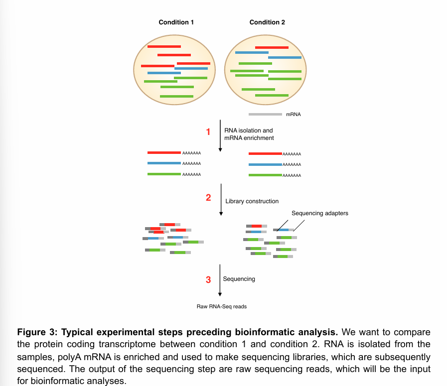
Typical experimental steps preceding bioinformatics analysis of transcriptomics experiment

After obtaining the samples you want to use for transcriptome analysis, the “pre-bioinformatics” part workflow can be divided into three components:

• RNA isolation and enrichment of the species of interest (mRNA in the figure).

• Library construction

• Sequencing

The output of this process (and thus the input of the bioinformatics analysis) are the raw RNA-seq reads.

RNA isolation

RNA isolation (or RNA extraction) is the process of purifying RNA from biological samples (we separate it from DNA and other molecules, for example).

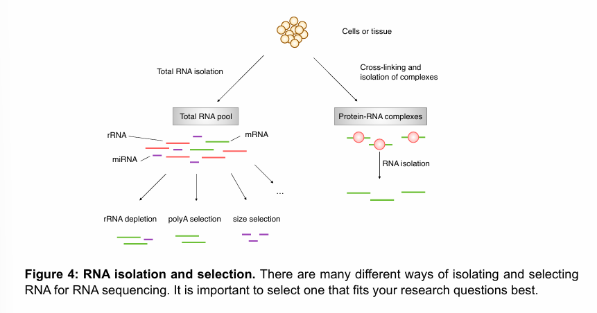
RNA selection

RNA selection refers to the process of enriching or isolating specific types of RNA molecules from total RNA before downstream applications like RNA sequencing (RNA-seq). This step helps focus on relevant RNA populations (e.g., mRNA, rRNA, non-coding RNA) and improves data quality and interpretation.

Example of methods to enrich samples for mRNA.

• PolyA selection: effective way to remove everything but mRNA and some minor RNA species with a polyA tail. This technique does not work for prokaryotes, as their mRNAs typically do not have a polyA tail.

• rRNA depletion: indirect way of increasing the abundance of mRNAs in sample. The sample will also contain non-mature mRNAs (with no polyA tail).

• Size selection: by selecting for small RNAs, the sample can be enriched for miRNAs, for example. Conversely, mRNAs are retained when selecting for larger fragments.

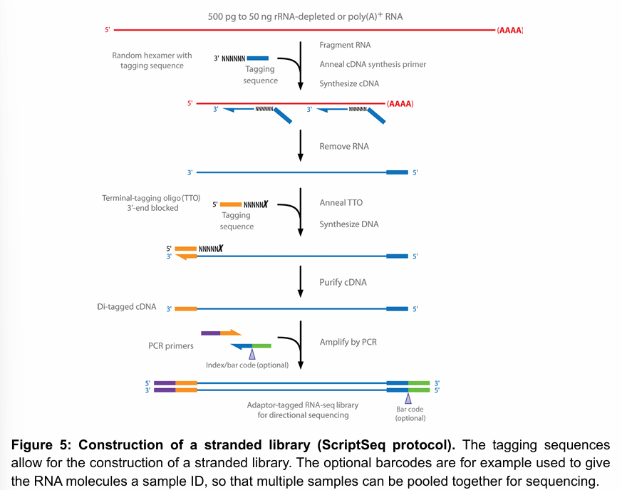
Briefly describe how library construction works in a transcriptomics workflow.

Library consists of DNA fragments of a specified length, representing the RNA pool, with sequencing adapters on both ends. Usually, library prep follows the following workflow:

• RNA fragmentation

• cDNA synthesis

• Addition of sequencing adapters

• PCR amplification

Figure shows an example of a protocol to make a stranded library.

Briefly describe how sequencing works in a transcriptomics workflow.

At this point in the workflow, we are working with DNA. Thus, the sequencing is done using similar technologies and protocols as those used for next-generation genome sequencing.

Overview of the bioinformatics analysis workflow in the transcriptomics.

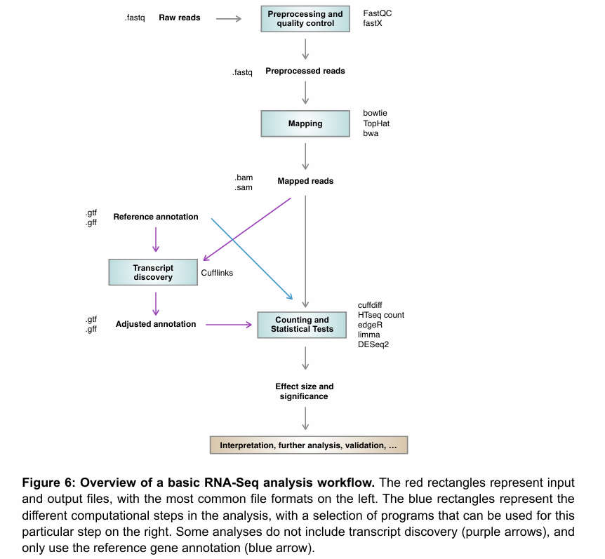
Describe the role of the pre-processing and quality-control step in the bioinformatics analysis workflow.

To solve the fact that:

• some reads will be of poor quality

• some reads can still contain adapter or vector sequences

• some sequences may be duplicated due to the PCR reaction

• reads can be biased with regards to their GC content or overall base content over the length of the read

• barcodes may be present (multiplexing)

• the end of reads tend to be of very poor quality

These aspects must be removed before analysis.

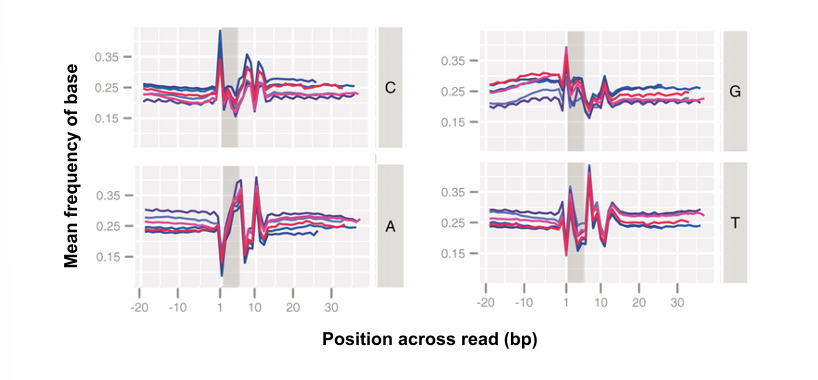
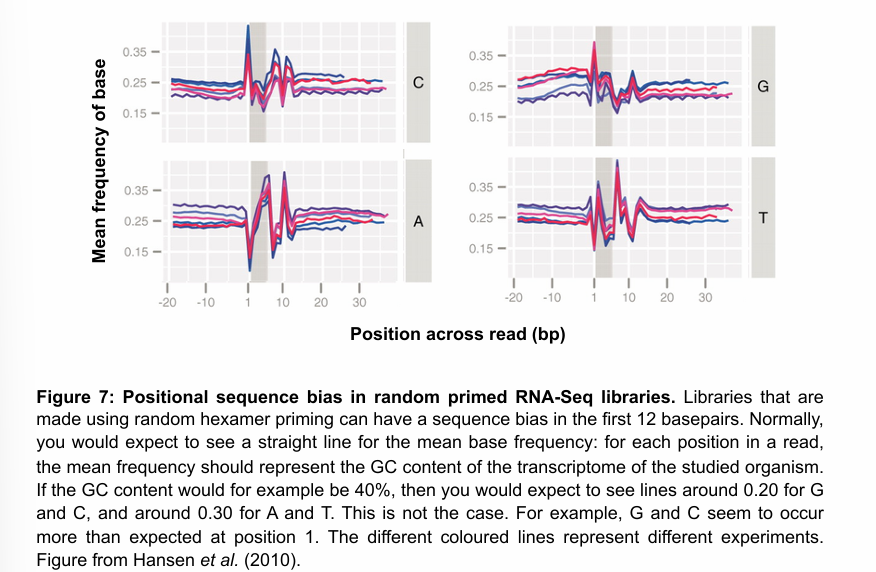
Explain what these graphs represent, and what must be done about it in a transcriptome analysis workflow

• These four graphs give the mean frequency of each base across all reads in an RNA-seq library, as a function of position in the reads. The different lines within one graph correspond to different experiments.

• Normally, we would expect these lines to be roughly constant with respect to position. More specifically, for each position in a read, the mean frequency of the bases should correspond with the GC content of the transcriptome of the studies organisms. For example, if the GC content of the organism is 40%, then we would expect a mean frequency of base of 0.20 for G and C, and 0.3 for A and T.

• However, we see that there is a bias around the first 12 positions (represented by the shaded areas).

• This bias arises because the library was built using random hexamer primers. As a result, the beginning of the reads in the library are biased towards these primers.

• This bias can be fixed in the pre-processing step of the bioinformatics workflow.

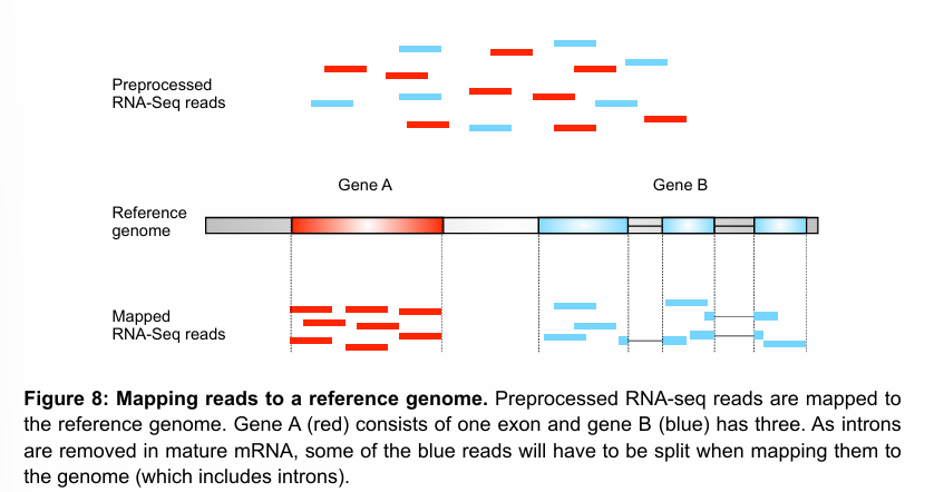
What are important things to consider when mapping RNA-seq reads to a genome?

• Splicing is very common in many eukaryotes. Thus, if mature mRNA is used to construct the libraries, the reads will only consists of exons. Thus, none of the reads will map to introns, and if a read contains an exon boundary, it will need to be split to be correctly mapped to the genome.

• Strandedness of the library has to be specified for the mapping to be carried out correctly.

De novo transcriptome assembly

De novo transcriptome assembly is the process of reconstructing the full set of RNA transcripts from short RNA-seq reads without a reference genome.

This is done by joining reads that overlap. No need to know the details of de novo sequencing for this course.

Output of mapping program

.bam and/or .sam

These two file types contain the same information, but sam is human readable, and bam is binary.

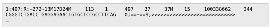
What is this? Explain all elements.

Entry in a .sam file.

In a sam file, each row is a separate entry (in the picture, the row spans two lines).

• Column 1: QNAME, unique name of the alignment (e.g. 1:497:R:-272+13M17D24M)

• Column 2: FLAG, describes alignment in code (e.g. 113 = this is the first read of a pair, both reads in the pair were flipped and both were mapped).

• Column 3: RNAME, name of reference sequence, often the chromosome (e.g. 1).

• Column 4: POS, leftmost position of where the alignment maps to the reference (e.g. 497).

• Column 5: MAPQ, mapping quality, similar to Phred (e.g. 37).

• Column 6: CIGAR, describes how many bases of the read matched (e.g. 37M = 37 bases matched; 3M1I3M1D would be 3 matches, 1 insertion, 3 matches 1 deletion).

• Column 7: MRNM/RNEXT, name of reference sequence of next alignment (e.g. 15; ‘=‘ if idem).

• Column 8: MPOS/PNEXT, position of next alignment (e.g. 100338662).

• Column 9: ISIZE/TLEN, length of leftmost mapped base to rightmost (e.g. 344).

• Column 10: SEQ, read sequence.

• Column 11: QUAL, Phred quality scores of the read.

Can a read have several entries in a .sam file? What does it mean?

Yes, a read can have several entries in a .sam file. It means that the read was mapped to several regions of the genome (multiple mapping). In this case, the mapping quality is lower?

Transcript discovery, and main tool used for it.

Process of identifying novel transcripts and isoforms from RNA-seq data. In other words, after mapping our reads to the reference genome, we identify regions in the genome where a lot of reads map, but with no annotations.

Main tool for transcript discovery is cufflinks.

Counting

After pre-processing and quality control, mapping, and potential transcript discovery, the next step is counting (and ensuing statistical tests).

Usually, this consists in:

1. Count the number of reads that fall in a certain interval (e.g. gene or exon).

2. Test is there is a significant difference between these number for different conditions.

In this step, the mapped reads (.bam or .sam) are used together with a gene annotation file (.gtf or .gff) to generate a list of all annotated genes with an estimate of their expression.

Example of a program that does this is HTseq.

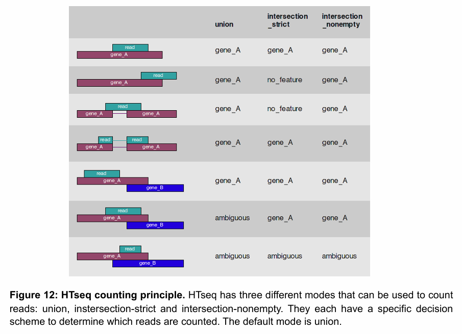
Explain how HTseq-count works, and what are the limitations

It applies different rules for ambiguous reads (those that overlap more than one gene or don’t fall entirely within a feature):

• Union (default): A read is counted for a gene if it overlaps any part of a gene’s exons and doesn't overlap another gene.

• Intersection-strict: A read is only counted if it falls entirely within a feature.

• Intersection-nonempty: A read is counted if some part of it overlaps a feature, even if it overlaps more than one.

This is a naïve way of counting which does not deal with isoforms very well.

Challenges with counting

Short reads may not span exon-exon junctions, so it is difficult to determine the exact isoform of origin. This can be solved by using longer reads, which is possible with next generation sequencing.

Program other than HTseq that estimates gene expression and deals with isoforms better.

Cuffdiff (from Cufflinks)

It uses two sources of information:

• reads that must have come from different isoforms

• the likelihood a fragment came from a particular isoform, based on the size of the sequenced fragments and isoforms.

What is the goal of normalisation in transcriptomics analysis.

One of the most common objectives in transcriptomics is to compare gene expression between different conditions. Using the expression estimates obtained in the previous step, statistical tests are carried out to determine which genes are significantly differentially expressed.

However, it would be incorrect to just take the raw count data as input for these tests. Each experiment, even if carried out perfectly, will contain a number of biases. This means that different samples, or even different genes within one sample cannot be directly compared with regards to their raw counts. The solution to this problem is normalisation.

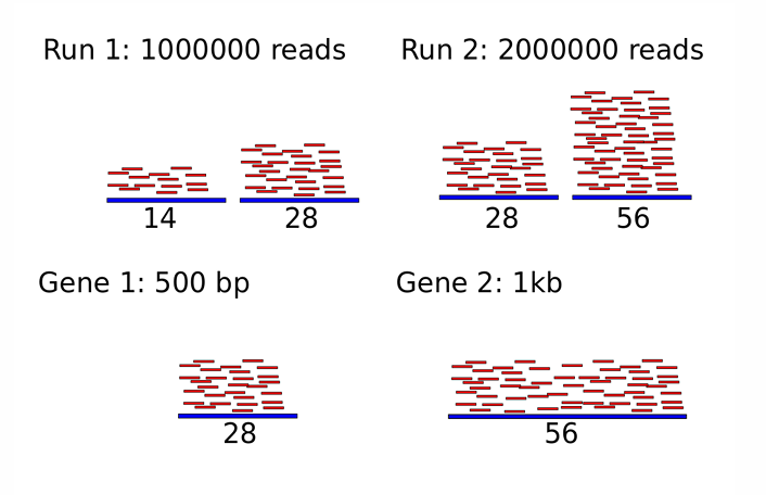
Most common sources of bias in RNA-seq

• Sequencing depth (between runs): The total number of reads differs between samples due to RNA/cDNA quality, library construction imperfections, or minor hybridisation deviations. If library sizes vary, raw gene counts are not directly comparable (see top of figure).

• Gene length (within library): Within a sample, gene length affects interpretation. For example, gene X with 20 reads over 2 kb and gene Y with 10 reads over 1 kb have similar expression when normalized for length. Longer transcripts naturally yield more reads at equal expression (see bottom of figure).

• Count distribution differences: A few highly expressed genes can dominate read allocation, reducing confidence in detecting changes in less-expressed genes. A change from 1000 to 2000 reads is more robust than from 1 to 2. Since read totals are limited, highly expressed genes increase uncertainty for others—hence the need to deplete rRNA.

Normalisation techniques

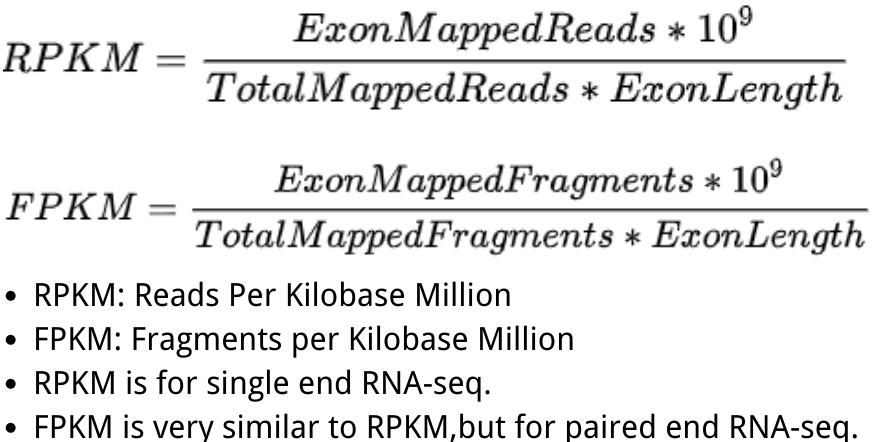
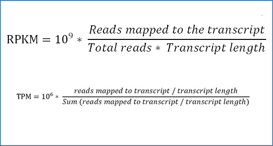
• RPKM/FPKM: Reads/Fragments per kilobase of transcript length per one million mapped reads/fragments.

• TPM: Transcripts per million.

• Total count

• Median

• Upper quartile

RPKM/FPKM

Reads/fragments per Kilobase of transcript length per one Million mapped reads/fragments.

First accounts for library size and then gene length.

Introduces a bias in per-gene variances

TPM

Transcripts per million

First accounts for gene length and then library size.

Allows direct gene comparisons between samples.

Why is it important to not only normalise for gene length and library size, but also for count distribution?

Normalisation methods that account for differences in count distribution

• TMM normalisation: trimmed mean of M values

• Geometric mean normalisation

TMM

Trimmed mean of M values

TMM tries to normalize expression counts between samples so that the majority of genes are not changing.

• The majority of genes (assumed not to be differentially expressed) will now show no fold change (M ≈ 0).

• It corrects for global shifts due to a few highly abundant transcripts.

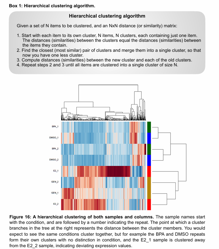
Two main approaches to globally compare samples?

1. Hierarchical clustering

2. PCA

Hierarchical clustering

Input is a matrix where the rows correspond to each gene, the columns correspond to samples, and the values are the gene expression levels for a given gene in a given sample (normalised).

Hierarchical clustering helps answer:

• Which genes have similar expression patterns across samples?

• Which samples show similar transcriptomic profiles?

Two decisions to make in hierarchical clustering:

1. How will the sample vectors (i.e. columns) be compared?

   • Euclidian distance

   • Pearson correlation

2. How will the clusters of samples be compared?

   • Centroid clustering

   • Average-linkage clustering

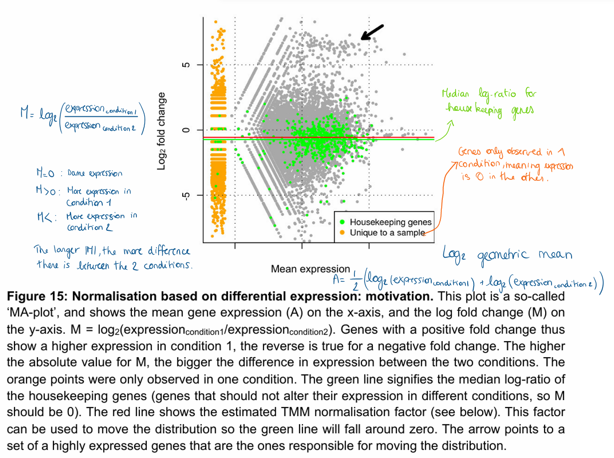
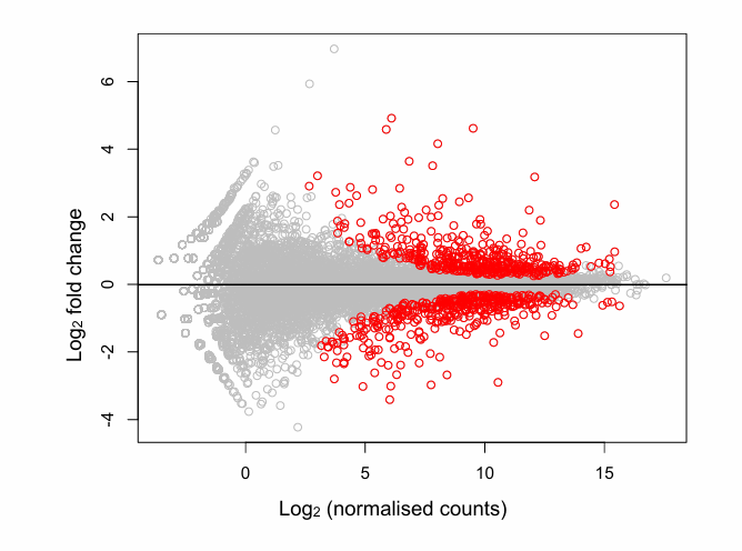
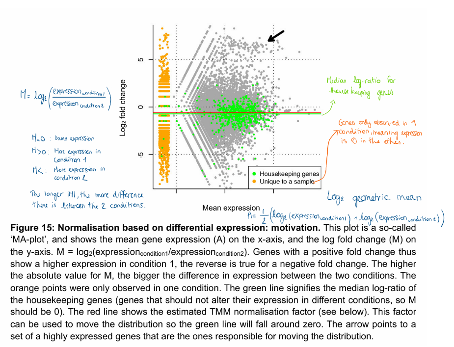
How to evaluate trends between abundance and effect in transcriptomics data?

MA plot

Abundance (A): x-axis → mean of the log2 normalised counts

Effect (M): y-axis → log2 fold change between two conditions

Plot can also highlight the results of the statistical tests by colouring the significant genes (dots) in a different colour (red in the figure).

Most important observations in MA plot?

1. Unexpected biases in the relation between the effects (y axis) and expression level (x-axis).

   For example, we would expect most of the genes to have no effect, so the mean to be close to a log2 fold change of 0 over the whole abundance range.

   Deviations from this could highlight problems with normalisation or an uncorrected bias.

2. Outliers, both in the sense of individual genes, or whole samples.

3. Shows from which level of expression we can expect to be able to identify differential expression.

How to evaluate trends between effects and levels of significance?

Volcano plot

• The higher the point, the lower the p-value (i.e. more significance)

• Fountain shape: larger effects, both positive and negative, will be associated with rejecting the null hypothesis at higher level of certainty (smaller p-values appear higher on the graph)

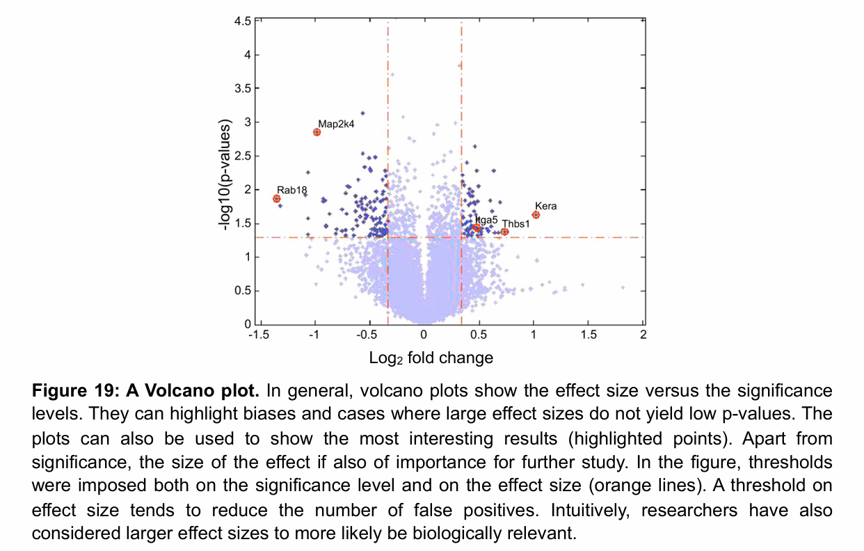
In a volcano plot, what does it mean if we observe genes with large effects but a lack of significance?

• These points will appear in the lower corner of the volcano plot (low because no significance → y-axis, in the corners because of large effect → x-axis).

• This indicates that there may be high variability in the measurements for replicates of the same conditions, thus leading to a lack of significance despite the large effect.

• This could reflect a problem in the data acquisition or processing !

How to evaluate if a gene is differentially expressed?

Statistical testing

• Values used as input should be the normalised counts

• For a given gene, the expression is average across replicates for two conditions → µ1 and µ2. Variability across replicates is also computed and very important in significance determination.

• H0: µ1 = µ2 and H1: µ1 ≠ µ2

• We basically test if any differences between two conditions can be explained by random variations.

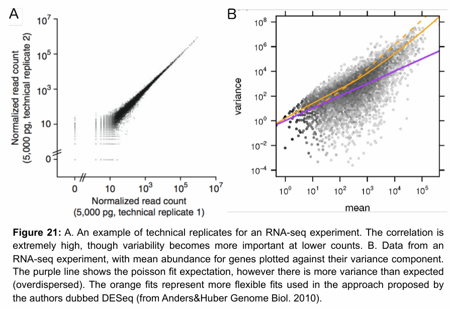
Good model for comparing between two conditions

Negative binomial distribution.

Poisson distribution can also be used, but it has been observed that RNA-seq data often shows overdispersion compared to Poisson (more variance). It works for technical replicates, but otherwise imperfect fit.

Negative binomial distribution is better because it can model both mean and variance independently. Poisson has only one parameter to estimate mean and variance → lambda. Negative binomial has an additional parameter.

Model formulation and hypothesis testing

Generalized linear model

log(µ) = beta_0 + x beta_1 + epsilon

x takes value 0 in one condition and 1 in the other. Thus, if beta_1 is 0, then there is no difference between the two conditions.

Statistical tests consists in checking if beta_1 is significantly different from 0. The p-value is given by the Wald test.

Source of variability between replicates

• Shot noise: random sampling errors, especially in low-abundance transcripts. Stochastic effect

• Technical noise: lab-based variability. Controllable and can be reduced by focusing on better laboratory practices.

• Biological noise: true biological variation across samples. Can be limited by having careful experimental design.

How to deal with shot noise?

• Deeper sequencing

• More material to generate sequencing library

• More replicates

Shot noise is dominant for … expressed gene.

lowly

Biological noise is dominant for … expressed gene.

strongly