3 ECON 201 - Midterm #2 (3/27/26)

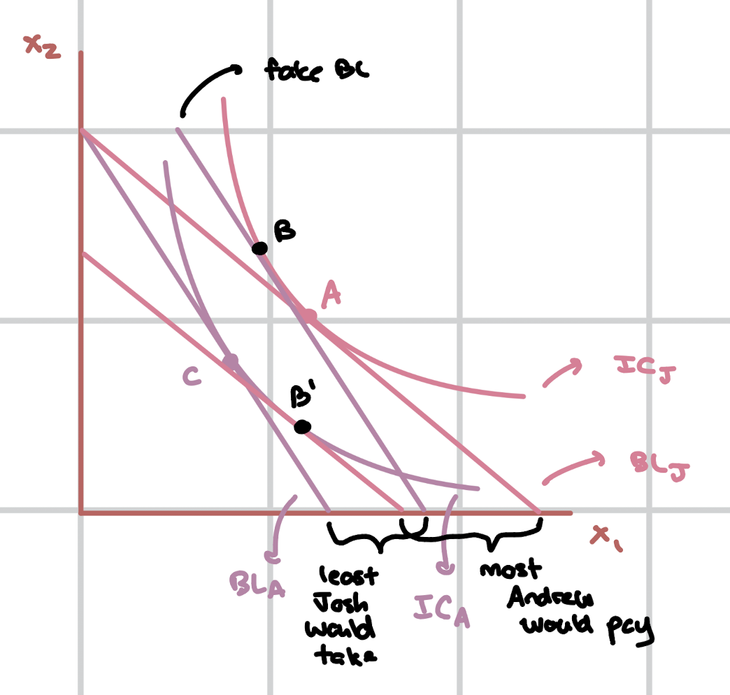
Taxes / Coupons

C → B: The least that Josh would take to be compensated for experiencing the tax / losing the coupon (CV).

A → B’: The most Andrew would pay to avoid experiencing the tax / experience the coupon (EV).

Compensating Variation (CV)

The amount of money a consumer requires to offset a loss in utility due to a tax or a loss of a coupon, reflecting their willingness to pay for a change in circumstance.

E(p₁^T, p₂, u^NT) - E(p₁^NT, p₂, u^NT)

Equivalent Variation (EV)

The maximum amount of money a consumer would be willing to pay to avoid a loss in utility from a tax or to attain a coupon, indicating their perceived value of a change in circumstance.

E(p₁^T, p₂, u^T) - E(p₁^NT, p₂, u^T)

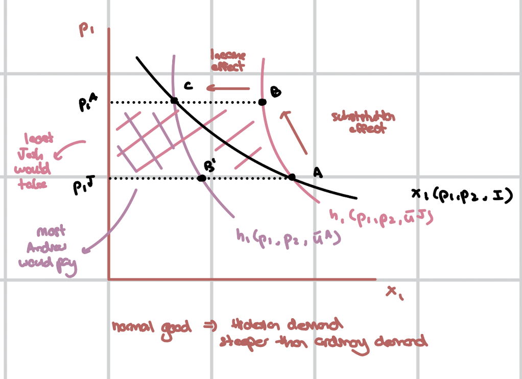
Inverse Demand Curves - Normal Good

Hicksian demand is steeper than ordinary demand.

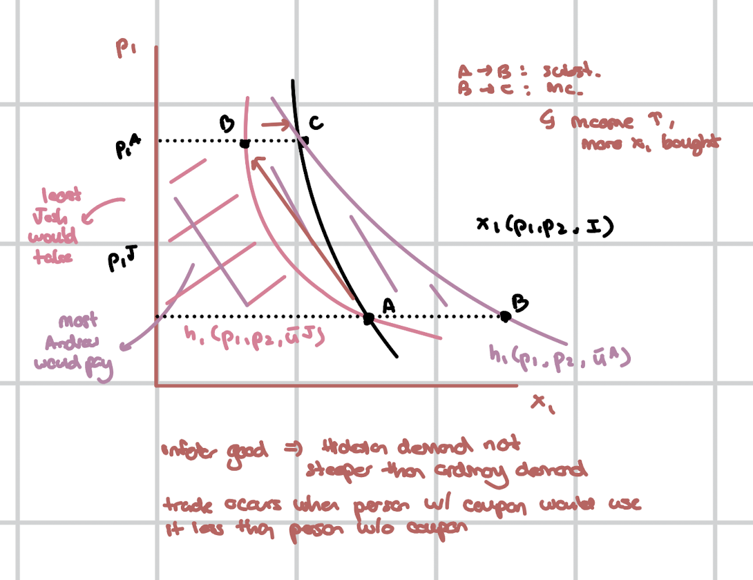
Inverse Demand Curves - Inferior Good

Hicksian demand is not steeper than ordinary demand.

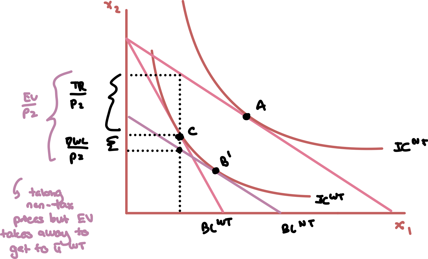
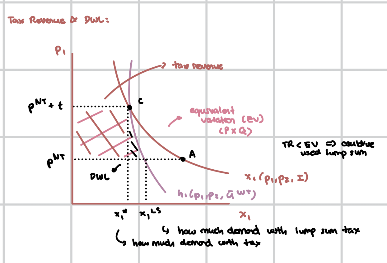
Tax Revenue & DWL

TR = t * x_1^*
EV = TR + DWL
Lump Sum Tax = Total of EV, no DWL

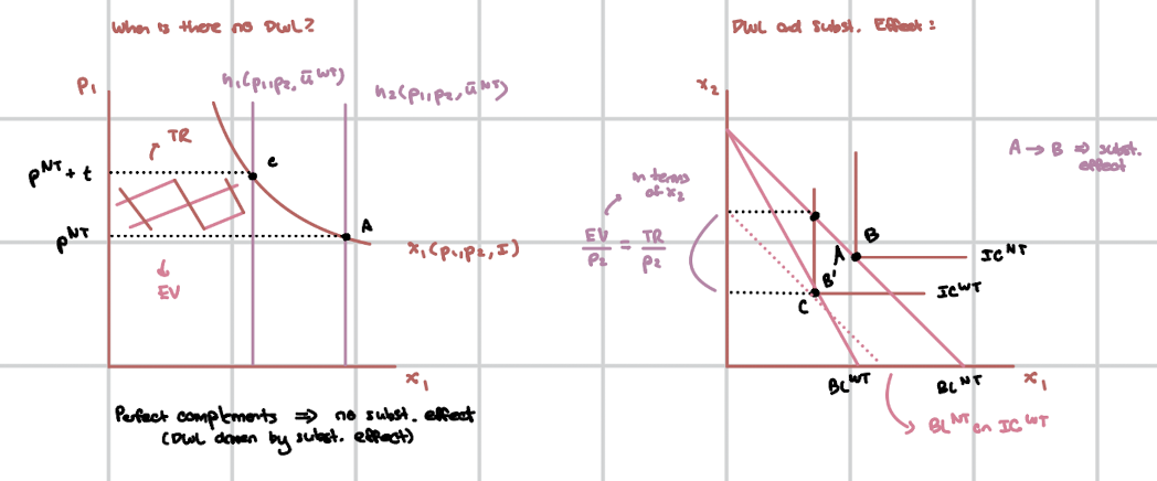
Tax Revenue & DWL - No DWL

Hicksian demand curves are vertical → perfect complements.
There is no DWL when demand is perfectly inelastic; DWL comes from the substitution effect; if they are perfect complements, there is no substitution possible.

EV = TR

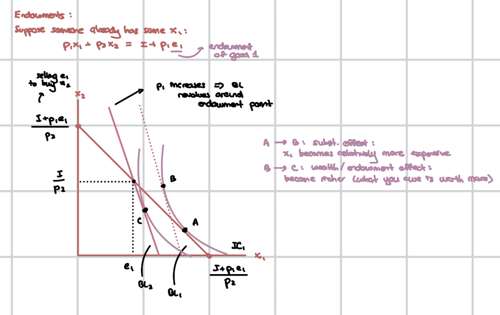
Endowments - Net Buyer

If p₁ Increases:

• Substitution Effect (A → B): x₁ becomes relatively more expensive, so consume less x₁

• Wealth / Endowment Effect (B → C): the rise in price of x₁ makes you wealthier, because you own it

Budget line always rotates around the endowment point (e₁, _)

• At the endowment bundle, you are not trading, so price changes do not affect your ability to consume that exact bundle.

Net Buyer (x₁ > e₁) → price increase makes you worse off → wealth effect reduces consumption.

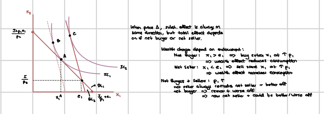
Endowments - Net Seller

Substitution effect always reduces the consumption of x₁ if p₁ increases.

Net Seller (x₁ < e₁) → price increase makes you better off → wealth effect increases consumption.

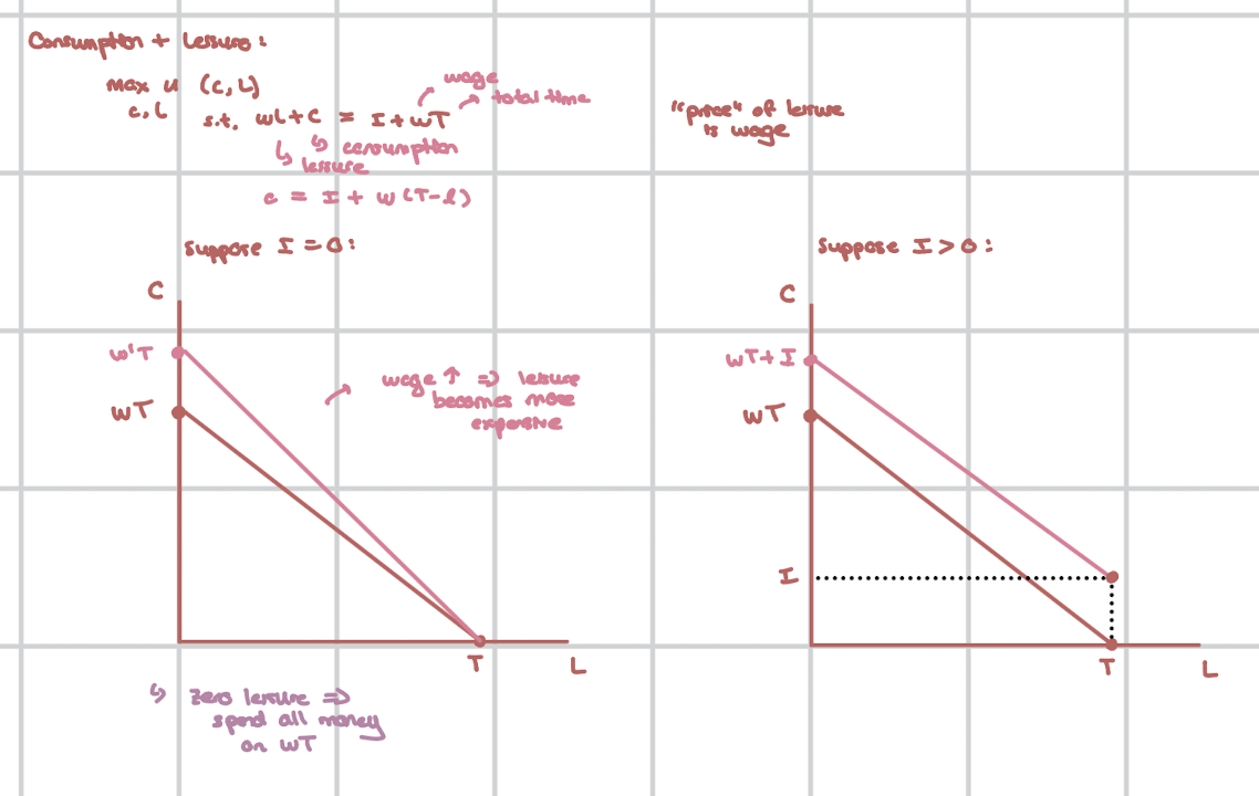
Consumption & Leisure

Budget Constraint:
wl + c = I + wT
c = I + w (T - l)

slope = -w
intercept (l-axis) = T
intercept (c-axis) = I + wT

If wage increases:

• Substitution effect → leisure more expensive, consume less leisure.

• Income effect → wage increases, you are wealthier; if leisure is a normal good, consume more leisure.

The total effect on leisure is ambiguous.

If you have Income > 0:

• at leisure = T (no work) → c = income

If substitution effect > income effect → labor supply decreases with wage decrease because leisure has increased.
If income effect > substitution effect → labor supply increases with wage decrease because leisure has decreased.

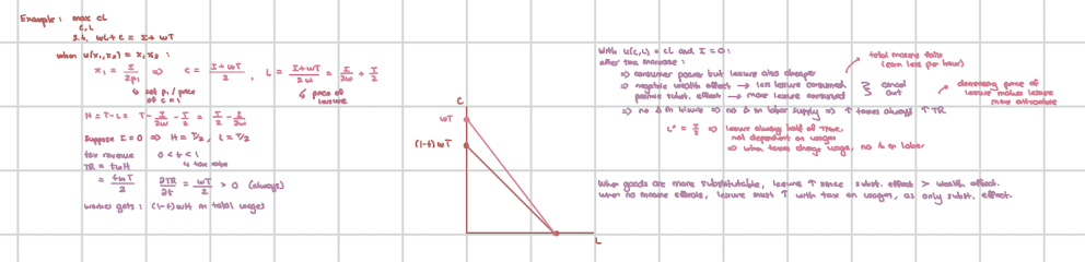
Tax on Wages

TR = twh

DWL comes from behavioral change, but because there is no substitution effect in this case (labor supply is fixed) there is no DWL.

If there is no income effect, then leisure increases with a decrease in wages.

Based on the utility function:

• If utility is linear in a good → no income effect for that good. If marginal utility doesn’t change with income, then the consumer's choices remain unaffected as income variations do not alter the quantity consumed.

The Laffer Curve → Shows TR as a function of the tax rate, t.

• The substitution effect is what reduces labor supply as taxes increase / wages fall (leisure becomes cheaper, so leisure increases).

• The income effect only affects what occurs based on whether leisure is a normal good or not (if normal, leisure will decrease as income decreases / taxes increase).

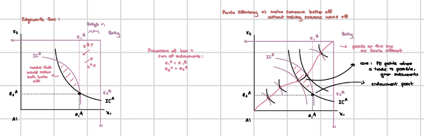
Edgeworth Box / Pareto Efficiency

Each point in the box is a feasible allocation.

A Pareto Efficient allocation occurs when no individual's situation can be improved without worsening another's situation. It represents an ideal distribution of resources between two individuals.

Points inside the lens are mutually beneficial trades.

Contract Curve → Where ICs are tangent (MRS¹ = MRS²). Some efficient points are very unequal (some give almost everything to one person).

The lens → all improvements over endowment.
Contract curve → all efficient allocations.
Core → part of contract curve inside the lens.

Efficient → No more gains from trade (no waste).
In the Core → Efficient and both prefer it to the endowment.

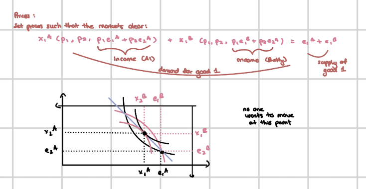
Edgeworth Box → Market Clearing

Demand = Supply

Set total demand for the good equal to total endowment (supply) for the good.
Solve for the ‘market clearing’ price ratio.
No excess demand, no excess supply, everything produced is consumed.

Equilibrium → Where both customers optimize and the market clears.
Plug the price ratio into the individual demand functions for each person to determine individual demands.

Welfare Theorems:

1. Every competitive equilibrium is Pareto efficient. No gains from trade remain. Markets lead to efficiency automatically.

2. Any Pareto efficient allocation can be achieved via markets (with transfers); you can redistribute endowments.

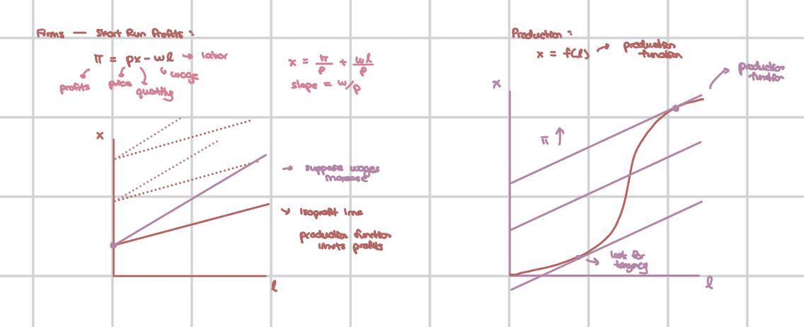
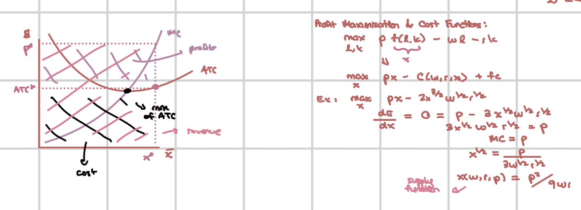
Profits

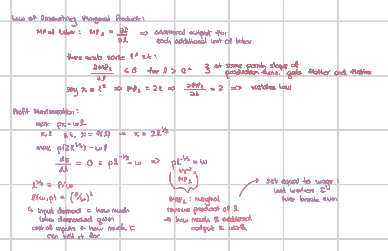
Law of Diminishing Marginal Product:

• MP_l = df / dl → dMP_l / dl < 0 → each additional worker adds less extra output (production function becomes flatter)

Input Demands → Properties

1. HD0 in prices (input and output)

2. Decreasing in own-input price

Supply Function → Properties

1. HD0 in prices (input and output)

2. Increasing in output price

3. Decreasing in input prices

Profit Function → Properties

1. HD0 in prices (input and output)

2. Increasing in output prices

3. Decreasing in input prices

4. Hotelling’s Lemma (taking derivative in terms of p → x(w,p); taking derivative in terms of w → -l(w,p))

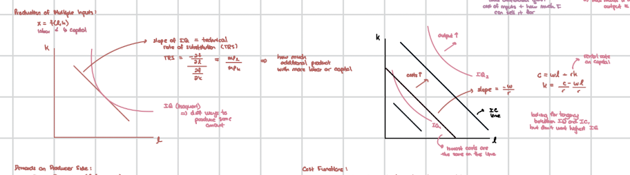
Production of Multiple Inputs

Isoquant → a curve that represents all combinations of inputs that yield the same level of output.

Marginal Rate of Technical Substitution (MRTS) = MP_l / MP_k = slope of IQ

Isocost → C = wl + rk

Corner Solutions:

1. On outputs → when f(l, k) is CRTS or IRTS; want to produce either 0 or to infinity.

2. On inputs → use only labor or capital when IQs are linear or bowed the wrong way.

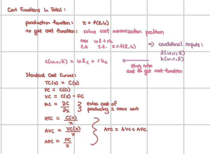
Cost Minimization

1. Solve a minimization problem of the cost function, subject to the production function for a particular output.

2. IQ slope = IC slope → (-df / dl) / (df / dk) = -w / r

Solve for l and k to get conditional input demands.
Plug in these demands into the cost function to get the cost function.

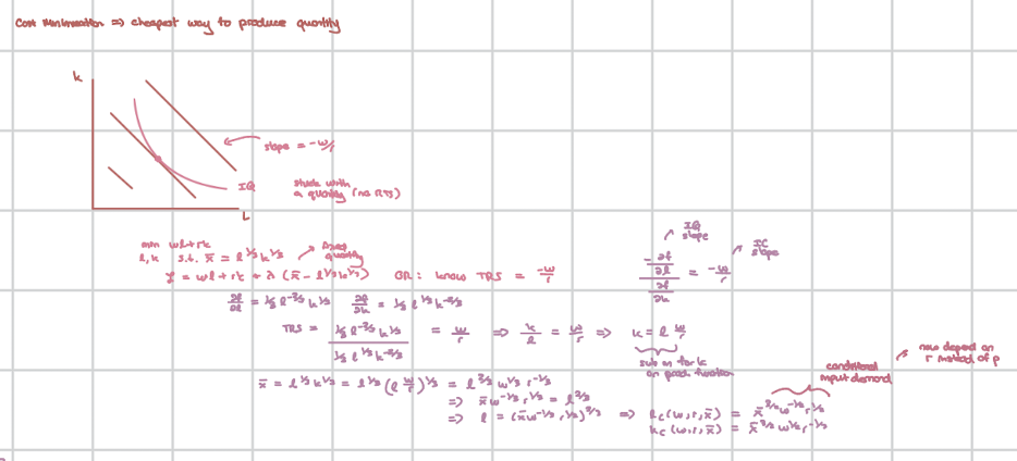
Conditional Input Demands → Properties

1. HD0 in input prices

2. Decreasing in own input price (dl / dw < 0, dk / dr < 0)

Cost Functions → Properties

1. HD1 in input prices

2. Increasing in input prices

3. Increasing in x

4. Shephard’s Lemma (take derivative of cost function in terms of w, get labor demand; take derivative of cost function in terms of cost of capital (r), get capital demand.

Standard Cost Curves

Cost Functions → Short Run

# of firms if fixed

Firms solve for profit maximization (px - cost function) subject to nothing. You’ll get p = MC.

Derive SR Supply:
Solve p = MC, solve for x as a function of p (firm individual supply).

Derive SR Demand:
x(p1, p2, I) → what one consumer demands
multiply by the # of consumers

Short Run Equilibrium:
Market Demand = Supply
Solve for equilibrium price p* and equilibrium market quantity x*.
Each firm produces x = x* / N.

Firms produce if p >= AVC.
SR supply = MC above AVC.

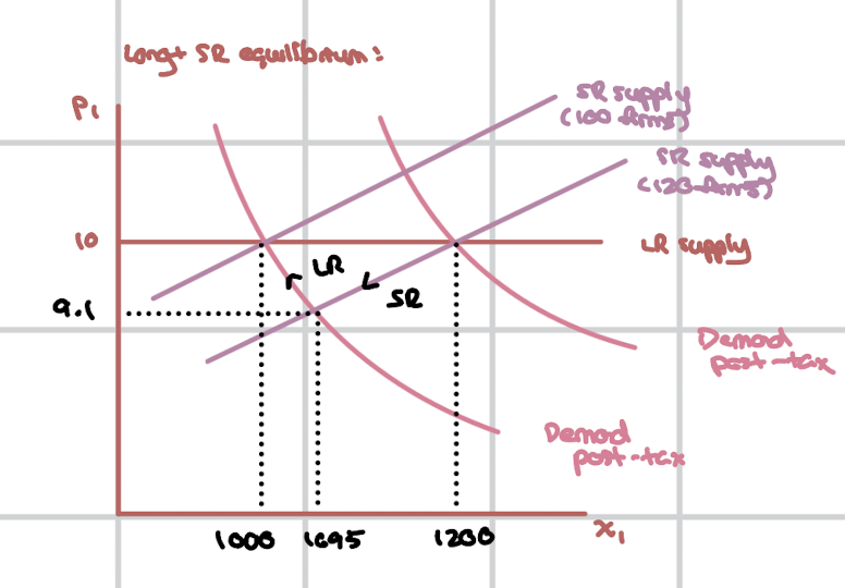
Cost Functions → Long Run

Firms enter / exit till profits = 0.

π = px - C(w, r, x) = 0
px = C(w, r, x)
p = ATC = MC

Derive LR Price:
Get optimal supply from p = MC.
Plug the supply into the profit function and set it equal to 0.
Solve for p*.
OR
dATC / dx = 0 → solve for minimizing output x*
p* = ATC(x*)

Derive LR Supply:
Solve for supply when profit equals 0 once optimal supply from P = MC is plugged in.

Long Run Equilibrium:
Market Demand = Supply
Find one firm’s output at the price: x* = x(p*).
# of firms = X* / x*