Statistics

Probability versus Inference

Probability models are the basis for understanding random phenomena, for which we repeat an experiment, but obtain a (slightly) different result.

Statistical inference is the science of drawing conclusions from experiments when the results could have come out differently if we repeated the experiment.

population

the entire collection of objects or outcomes about which we are seeking information

sample

a subset of a population, containing the objects or outcomes that are actually observed

simple random sample (SRS)

a sample of size n is a sample chosen by a method where each collection of n population items is equally likely to comprise the sample

conceptual population

a population that consists of all the values that might possibly have been observed

independence in a sample

The items in a sample are independent if knowing the values of some of the items does not help to predict the values of the others.

Items in a simple random sample may be treated as independent in many cases encountered in practice. The exception occurs when the population is finite and the sample comprises a substantial fraction (more than 5%) of the population.

one-sample experiment

an experiment where there is only one population of interest, and a single sample is drawn from it

multisample experiment

an experiment where there are two or more populations of interest, and a sample is drawn from each population

factorial experiment

a multisample experiment where the populations are distinguished from each other by the varying of one or more factors that may affect the outcome

numerical/quantitative data

data with a numerical quantity designating how much or how many is assigned to each item in a sample

categorical/quantitative data

data where sample items are placed into categories, and category names are assigned to sample items

controlled experiment

an experiment where the values of the factors are under the control of the experimenter in order to produce reliable information about cause-and-effect relationships between factors and response

observational study

an experiment where the experimenter simply observes the levels of the factor as they are, without having any control over them

sample mean

the arithmetic mean or average of the observations in the sample (the sum of the numbers in the sample divided by how many values there are); a measure of where the “center” of the data set is

deviation

the distance of a data value from the sample mean

sample variance

an adjusted average of the squared deviations

sample standard deviation

the (positive) square root of the sample variance

outlier

a data point that is either much larger or smaller than the rest of the data (because of measurement error, data entry error, or just because it’s different); in general values more than 1.5 x IQR from the closer of Q1 and Q3

sample median

the middle number in a data set

quartile

the quartiles divide the data set into quarters

• first quartile, Q1: the data value in position (0.25)(n + 1)

• third quartile, Q3: the data value in position (0.75)(n + 1)

interquartile range (IQR)

the measure of variability that is associated with the quartiles

IQR = Q3 - Q1

robust statistic

a statistic where removing the outliers does not change its value very much

stem-and-leaf plot

1. Select one or more leading digits for the stem values. The trailing digits become the leaves.

2. List possible stem values in a vertical column.

3. Record the leaf for every observation beside the corresponding stem value.

4. Indicate the units for the stems and leaves someplace in the display.

histogram

1. Divide the variable into discrete regions that partition the possible values of the variable, called classes, and construct class intervals of equal width.

2. Determine the frequency and relative frequency for each class.

3. Mark the class boundaries on the horizontal axis.

4. Above each class interval, draw a rectangle whose height is the frequency or relative frequency.

relative frequency

the relative frequency of a value is the proportion of units that have that value

When examining the distribution of data, what four aspects must we describe?

1. Shape

   1. Modes: unimodal, bimodal, or multimodal?

   2. Symmetry: symmetric, right-skewed, or left-skewed?

2. Center (e.g., mean or median)

3. Variability (e.g., standard deviation or IQR)

4. Outliers (unusual observations)

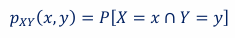
right-skewed (positively skewed)

lower values of the variable are more common with fewer and fewer observations having larger values of the variable; the right “tail” of the distribution is longer than the left tail

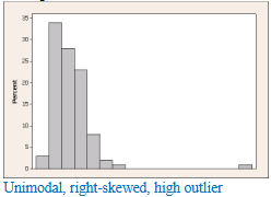
left-skewed

higher values of the variable are more common with fewer and fewer observations having smaller values of the variable; the left “tail” of the distribution is longer than the right tail

five-number summary

1. minimum

2. first quartile

3. median

4. third quartile

5. maximum

boxplot

graphical display of the five-number summary:

1. minimum

2. first quartile

3. median

4. third quartile

5. maximum

extreme outlier

in general, an outlier more than 3 x IQR from the closer of Q1 and Q3

How do we choose which values to use to describe the center and variability of a distribution?

• unimodal and roughly symmetric: use mean and standard deviation

• skewed and/or has outliers: use median and IQR (or the five-number summary)

experiment

a process that results in an outcome that cannot be predicted in advanced with certainty

sample space, S

the set of all possible outcomes of an experiment

event, E

a subset (collection) of outcomes from the sample space

simple event

an event with exactly one outcome

compound event

an event with more than one outcome

null event

an event with no outcomes

complement of an event

denoted A^C (for an event A), is the event that consists of all outcomes of S that are not in A

union of events

denoted A ∪ B, is the event consisting of all outcomes that are in at least one of the events A or B

intersection of events

denoted A ∩ B, is the event consisting of all outcomes that are in both of the events A and B

mutually exclusive events

events that never occur together: A ∩ B = ∅

exhaustive events

events where their union is the entire sample space: A ∪ B = S

probability

the probability of an event A, written P(A), is the proportion of times that event A would occur in the long run if the experiment were repeated over and over again under the same experimental conditions

probability model P( )

a function that satisfies the following axioms:

1. P(S) = 1

2. For any event A, P(A) ≥ 0

3. If events A₁, A₂, … are mutually exclusive, then P(A₁ ∪ A₂ ∪ …) = P(A₁) + P(A₂) + …

complement rule

for any event A, P(A^C) = 1 - P(A)

general addition rule

for two events A and B, P(A ∪ B) = P(A) + P(B) - P(A ∩ B)

(if A and B are mutually exclusive, then P(A ∪ B) = P(A) + P(B))

the conditional probability of event A given that event B has occurred

P(A|B) = P(A ∩ B) / P(B)

(this provides another method for computing P(A ∩ B), which is the general multiplication rule: P(A ∩ B) = P(B)*P(A|B)

independent events

two events A and B are independent if

• P(A|B) = P(A)

• P(B|A) = P(B)

• P(A ∩ B) = P(A)P(B)

(if one is true, they are all true)

mutually independent events

events A₁, A₂, …, A_n are mutually independent if the probability of each remains the same no matter which of the others occur

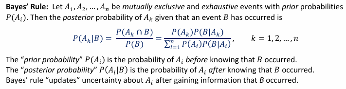
law of total probability

if A₁, A₂, …, A_n are mutually exclusive and exhaustive events, and B is any event, then P(B) = P(A₁ ∩ B) + … + P(A_n ∩ B)

equivalently, P(B) = P(A₁)P(A₁|B) + … + P(A_n)P(A_n|B)

prior probability

the prior probability P(A_i) is the probability of A_i before knowing that B occurred

posterior probability

the posterior probability P(A_i|B) is the probability of A_i after knowing that B occurred

Bayes’ Rule

the posterior probability of A_k given that event B has occurred

random variable

A random variable (RV) assigns a numerical value to each outcome in a sample space. It is customary to denote random variables with uppercase letters

discrete random variable

A random variable is discrete if its set of possible values is a finite or countably infinite set of individual points. This means that if the possible values are arranged in order, there is a gap between each value and the next one.

distribution of a random variable

A distribution of a random variable describes the values that the variable can take on and the probabilities that it takes on those values.

probability mass function

The probability mass function (pmf) of a discrete random variable 𝑋 specifies the probability that a random variable 𝑋 takes on value 𝑥:

𝑝(𝑥) = 𝑃(𝑋 = 𝑥)

• for any real x, p(x) = 0

• the sum of p(x) for all x = 1

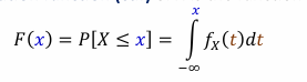
cumulative distribution function

The cumulative distribution function (cdf) of a random variable 𝑋 specifies the probability that a random variable 𝑋 takes on a value that is less than or equal to 𝑥:

𝐹(𝑥)=𝑃(𝑋 ≤ 𝑥).

Note: For a discrete random variable, the graph of 𝐹(𝑥) consists of a series of horizontal lines (called “steps”) with jumps at each of the possible values of 𝑋. The size of the jump at any point 𝑥 is equal to the value of the probability mass function 𝑝(𝑥) at that point 𝑥𝑥.

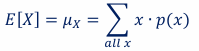
mean of discrete random variable

the sum of x*p(x) for all x

The mean of X is sometimes called the expectation or the expected value of X.

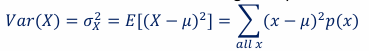
variance of a discrete random variable

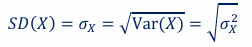
standard deviation

The standard deviation is the (positive) square root of the variance:

continuous random variable

A random variable is continuous if its set of possible values is an interval (with finite or infinite endpoints)

For any continuous random variable X and any number c, 𝑃(𝑋 = 𝑐) = 0

probability density function

Distribution of a continuous random variable is described by the probability density function (pdf), denoted by 𝒇(𝒙), where probabilities for a continuous random variable are the areas under the pdf

• the integral from negative infinity to infinity of a pdf is 1

• f(x) >= 0 for all x

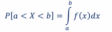
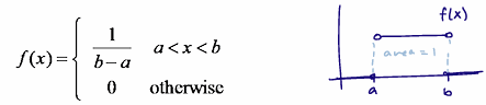
uniform distribution

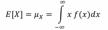
mean of a continuous random variable

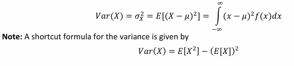
variance of a continuous random variable

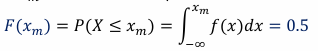
median of a continuous random variable

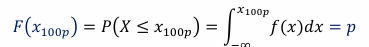
100p^th percentile

if 𝑝 is a number between 0 and 1, the 100pth percentile is the point 𝑥_100p that solves the equation:

jointly distributed random variables

When two or more random variables are associated with each item in a population, the random variables are said to be jointly distributed.

If all the random variables are discrete, they are said to be jointly discrete. If all the random variables are continuous, they are said to be jointly continuous.

joint probability mass function

If X and Y are jointly discrete random variables, the joint probability mass function (joint pmf) is:

• for all (x,y), p_XY(x,y) >= 0

• the sum of all p_XY(x,y) for all (x,y) = 1