AP Micro Unit 3 - Production, Cost, and the Perfect Competition Model

Production

* The process by which a producer takes inputs (factors of production) and creates an output

Fixed Costs

• The costs that aren’t affected by the quantity produced

• Examples:

  • Rent

Variable Costs

• The costs that are affected by the quantity produced

• Examples:

  • Tomatoes to make pizza sauce

Total Revenue

• Total amount of money a firm brings in

• TR = P * Q

Accounting Profit

• The amount of money a business makes

• Just explicit costs

Economic Profit

• Profit, including the opportunity cost

• Explicit and implicit costs

Total Product (TP)

• How much a firm outputs in total

• Example: 2 workers produce 50 units, total is 50

Average Product (AP)

• Divides total product by number of inputs

• Example: 2 workers produce 50 units, average is 25

Marginal Product (MP)

• Additional output from adding one more input

• Helps us determine when we should stop adding more inputs - zero or negative, we stop

• Example: 2 workers produce 50 units, 3 workers produce 60 units - the 3rd worker’s MP was 10 units

Law of Diminishing Marginal Product

* As we add more inputs, the additional product produced we get from each input will eventually diminish

Returns to Scale

• Proportional increase in output from an increase in inputs

• Production doubles when input doubles

Increasing Returns to Scale

* Production more than doubles with doubled input

Decreasing Returns to Scale

* Production less than doubles with doubled input

Short-Run

* Period of time where at least one input is fixed and cannot change

Long-Run

* Period of time where no variables are fixed

Accounting Costs

* Explicit costs paid by firms to use resources during the production process

Economic Costs

* Sum of both the implicit costs (opportunity costs) and explicit costs of production

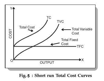
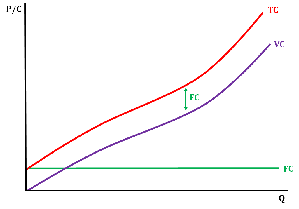
Total Cost

• Total cost of producing some quantity of output

• Sum of the variable and fixed costs

  • TC = VC + FC

Cost Curves Graph

Profit

• Difference of revenue and costs

• Profit = TR - TC

Average Total Cost (ATC) Equation

• TC / Q

• AFC + AVC

Average Variable Cost (AVC) Equation

• VC / Q

• ATC - AFC

Average Fixed Cost (AFC) Equation

• FC / Q

• ATC - AVC

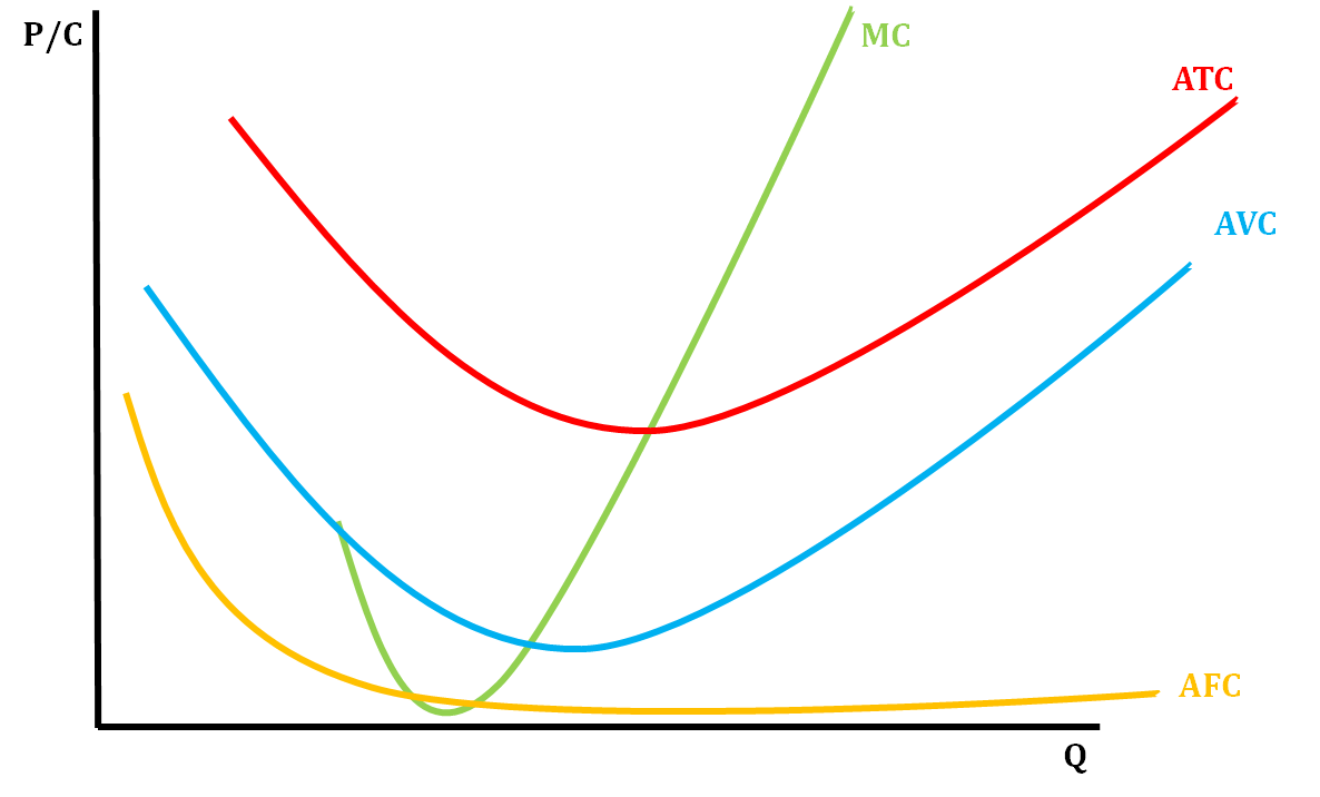
Marginal Cost

* Additional cost of producing one more unit

Total Cost, Variable Cost, Fixed Cost curves

MC, ATC, AVC, AFC curves

In the long run, all resources are…

flexible

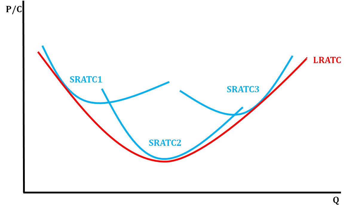
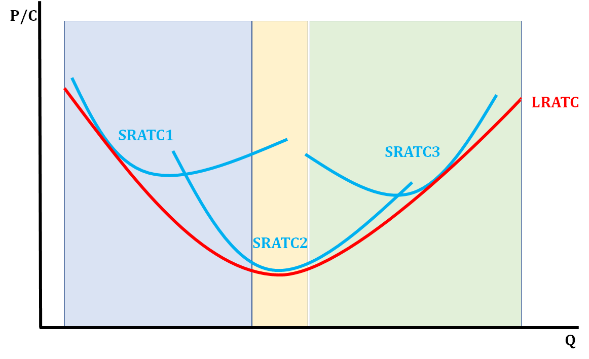
Long Run ATC (LRATC) Curve

* Short Run Total Cost Curves will shift in the Long Run as more is produced

How do we find Long Run ATC (LRATC)?

* Take the lowest average total cost curve at each level of output (short run cost curves)

LR ATC Car Scenario (to help understand)

• In the beginning of production, a factory does not use it’s full plant capacity and mass production is difficult, so there is a high cost producing less quantity

• As the firm continues production, it expands in capacity and can mass produce, lowering ATC

• As the firm expands, its output becomes larger than its plant capacity and is too big to manage, so costs rise again

Economies of Scale

• Refers to the reduction in total cost-per-unit as a firm increases its production

• In this phase, the firm can reduce the total cost-per-unit by boosting its plant capacity and output

Diseconomies of Scale

• Refers to the rise in total cost-per-unit as the firm increases its production

• In this phase, the firm would be better off reducing its plant capacity and output to lower per-unit costs

Constant Returns to Scale

• Between Economies of Scale and Diseconomies of Scale

• In this phase, when the firm increases production, costs stay the same

• ATC is at its lowest

Economies/Diseconomies of Scale

• Blue is Economies of Scale

• Green is Diseconomies of Scale

• Yellow is Constant Returns to Scale

What does each color represent in the graph:

• Blue

• Yellow

• Green

• Blue = Economies of Scale

• Yellow = Constant Returns to Scale

• Green = Diseconomies of Scale

Normal Profit

• When economic profit is zero - breaking even

• Our accounting profit is positive

Economic losses

* When revenue is less than costs

Supernormal profit

* When a firm experiences economic profits in the long run

Theory of the Firm

* The primary goal of any firm, regardless of market structure, is to maximize profits

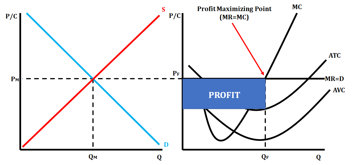
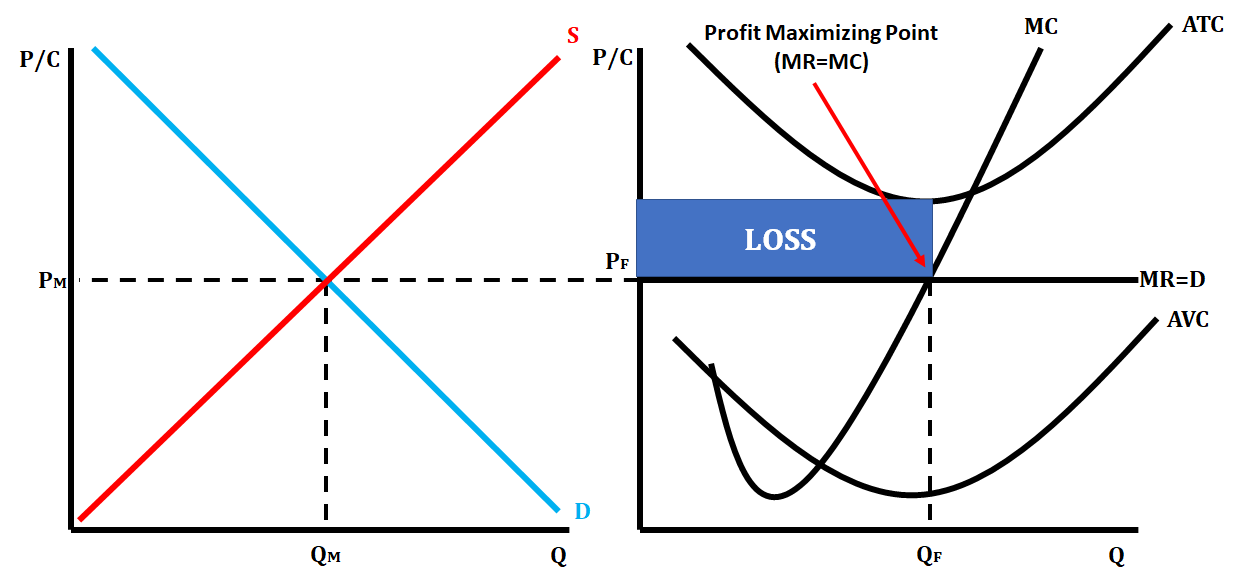
Profit Maximizing Rule

* MR=MC

Perfectly Competitive Market

• Many, small firms in the industry

• Firms are price takers, and have no control over the price of the goods they sell in the market

  • Market is impacted when firms enter or exit

• Low barriers to entry

• Firms break even in the long run

• Products sold are identical

• No non-price competition

  • All products are identical, so no need for advertising

• Firms are perfectly efficient in the long-run

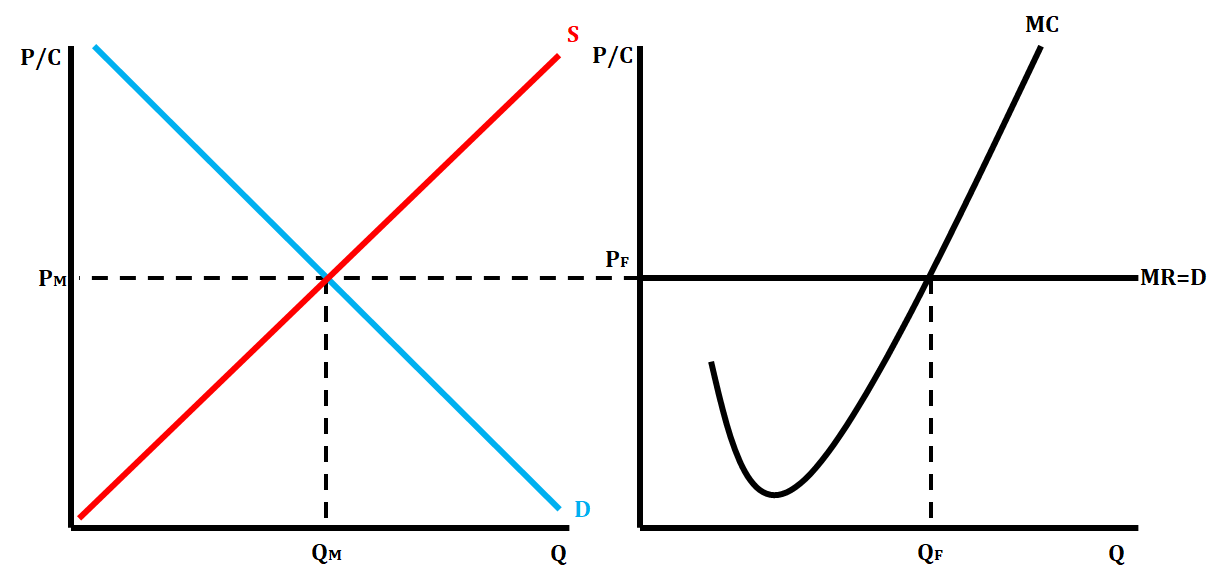
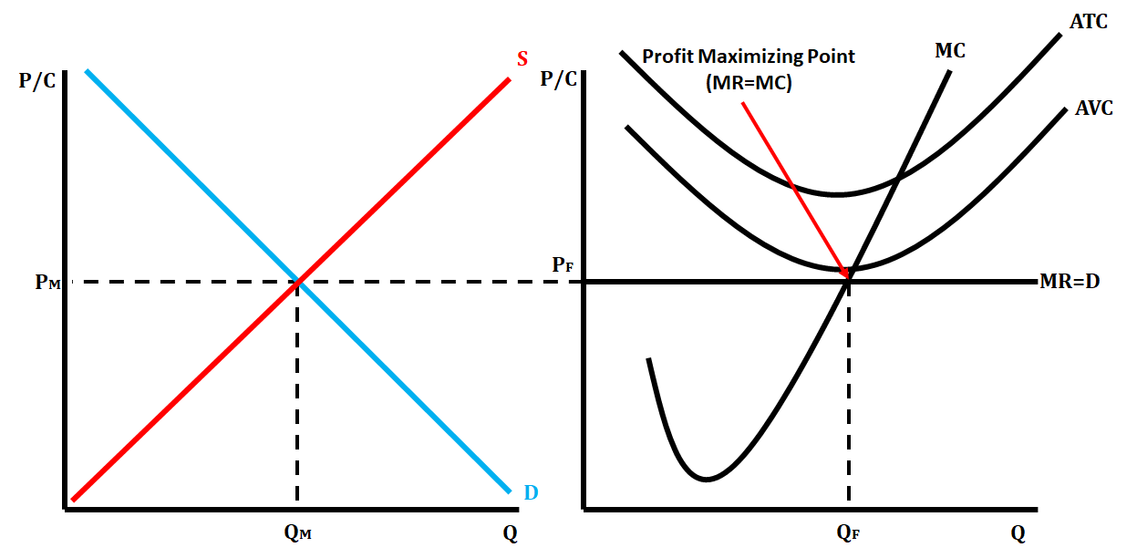
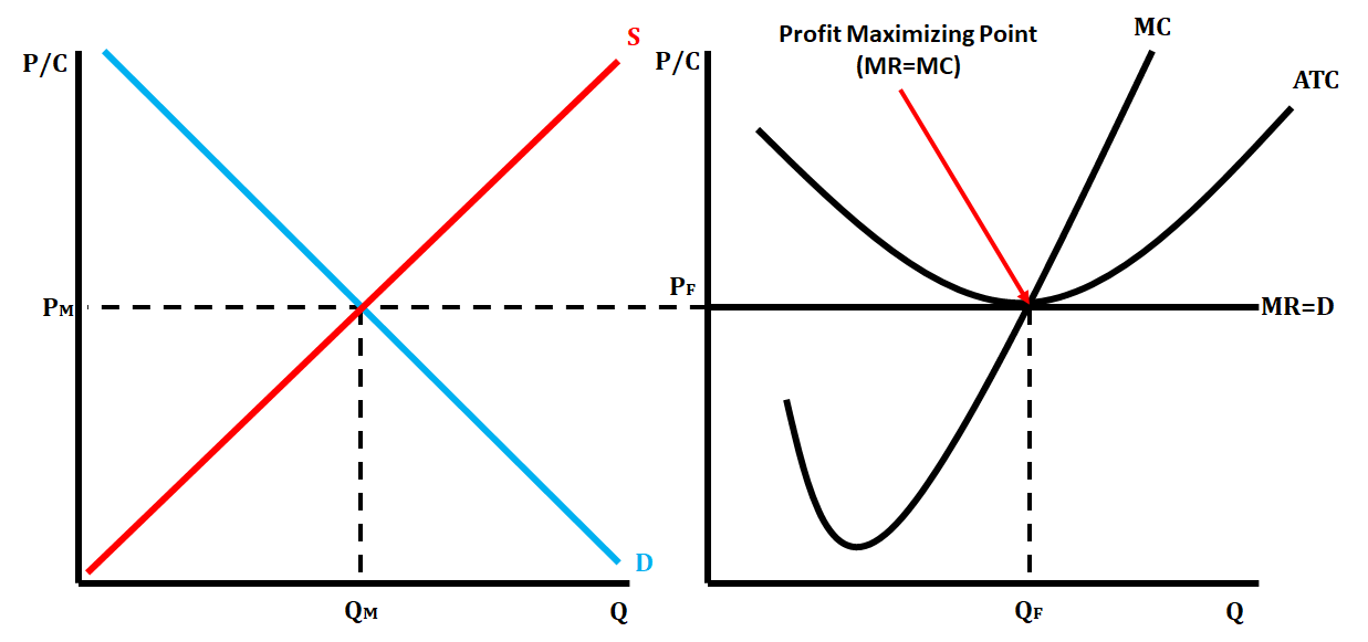
Perfect Competition Side by Side Graphs

Perfect Competition Short Run Profit

* ATC and AVC curves are below MR=MC

Perfect Competition Short Run Loss

* ATC curve is above MR=MC, and AVC curve is below MR=MC

Perfect Competition Short Run Shut Down

* ATC and AVC curves are above MR=MC

Perfect Competition Long Run Equilibrium

• ATC Curve is tangent to MR=DARP where MR=MC

• It is allocatively and productively efficient - perfectly efficient

Perfectly Competitive Market

Short Run Shut Down Rule

* The firm should continue to operate as long as the price is equal to or above AVC

Perfectly Competitive Market

When firms are earning economic loss in the short run, in the long run firms will…

leave the industry due to the lack of profit available

Perfectly Competitive Market

When firms are earning economic profit in the short run, in the long run firms will…

enter the industry due to the potential profit available

What is MR DARP?

MR = D = AR = P

* Market equilibrium is equal to marginal revenue

Perfectly Competitive Market

When a firm enters the market, what will happen?

• Supply will shift right

• This will decrease price, driving MR DARP down

Perfectly Competitive Market

When a firm leaves the market, what will happen?

• Supply will shift left

• This will increase price, raising MR DARP up

Perfectly Competitive Market

In the long run, the market will shift towards…

equilibrium, or normal profits