Business Analytics terms

nominal scale

nominal scale

classifies data into distinct categories with no ranking

ordinal scale

classifies data into distinct categories with ranking

population

contains all of the items or individuals of interest that you seek to study

sample

contains only a portion of a population of interest

population parameter

a number that summarizes the value of a specific variable for a population

sample statistic

a number that summarizes the value of a specific variable for sample data

simple random sample

every individual or item from the frame has an equal chance of being selected

• either with or without replacement

stratified sample

• divide population into two or more subgroups (strata) according to some common characteristics

• a simple random sample is selected from each subgroup, with sample sizes proportional to strata sizes

• samples from subgroups are combined into one

• even representation of population

cluster sample

• divide population into several “clusters,” each representative of the population

• select a simple random sample of clusters

summary table

tallies the frequencies or percentages of items in a set of categories so that you can see differences between categories

contingency table

• helps organize multiple categorical variables

• used to study patterns that may exist between the responses of two or more categorical variables

central tendency

the extent to which all the data values group around a typical or central value

mean

• most common measure of central tendency

  • affected by outliers

median

• middle number in an ordered array

• less sensitive to outliers than mean

range

• simplest variation measure

• sensitive to outliers

= largest # - smallest #

sample variance

a measure of the degree to which the numbers in a list are spread out

sample standard deviation

• most commonly used measure of variation

• is square root of variance

Z-score (aka standard score)

gives you an idea of how far a data point is from the mean

• data point is an extreme outlier if this is less than -3.0 or greater than +3.0

• the larger the absolute value of this, the farther the data point is from the mean

left-skewed distribution

• (median - smallest #) > (largest # - median)

• (Q1 - smallest #) > (largest # - Q3)

• (median - Q1) > (Q3 - median)

symmetric distribution

• (median - smallest #) ≈ (largest # - median)

• (Q1 - smallest #) ≈ (largest # - Q3)

• (median - Q1) ≈ (Q3 - median)

right-skewed distribution

• (median - smallest #) < (largest # - median)

• (Q1 - smallest #) < (largest # - Q3)

• (median - Q1) < (Q3 - median)

covariance

measures the direction of the linear relationship between two numerical variables

• cov(X,Y) is positive: X and Y tend to move in the same direction

• cov(X,Y) is negative: X and Y tend to move in opposite directions

• cov(X,Y) = 0: No linear relationship between X and Y

coefficient of correlation

measures the relative strength and directoin of the linear relationship between two numerical variables

• population variable: p

• sample variable: r

• closer to -1: stronger negative linear relationship

• closer to 1: stronger positive linear relationship

• closer to 0: weaker linear relationship

sample space

all possible outcomes of a variable

simple event

event with 1 characteristic

joint event

event with 2+ characteristics

complement

outcomes that are not part of an event

mutually exclusive events

events that cannot occur simultaneously

collectively exhaustive

a set of events is this if at least one of the events must occur

simple probability

the probability of a single event

joint probability

the probability of two or more events occurring simultaneously

marginal probability

consists of a set of joint probabilities while focusing on one variable

• you want to find the probability of a certain event as unconditioned by any other event

general addition rule

used to find the probability of either A or B

conditional probability

the probability that event A happens given information about event B

• P(A | B) = P(A and B) / P(B)

independent

events are this when the probability of one event is not affected by the fact that the other event has occurred

• if and only if: P(A | B) = P(A)

multiplication rule

used to find the probability events A and B occurring

marginal probability with multiplication rule

used to find the unconditioned probability of an event when the given events are mutually exclusive and collectively exhaustive

counting rule 1

If any one of k different mutually exclusive and collectively exhaustive events can occur on each of n trials, the number of possible outcomes is equal to k^n

• ex.: rolling a die 3 times

  • 6 sides

  • roll 3 times

  • 6³ = 216 possible outcomes

counting rule 2

If there are k₁ events on the first trial, k₂ events on the second trial, … and k_n events on the nth trial, the number of possible outcomes is (k₁)(k₂)…(k_n)

• ex.: you want to go to a park, eat at a restaurant, and see a movie. there are 3 parks, four restaurants, and 6 movie choices. how many diff possible combinations are there?

  • (3 parks)(4 restaurants)(6 movies) = 72 possible combinations

counting rule 3

the number of ways that n items can be arranged in order

n! = (n)(n-1)(n-2)…(1)

• ex.: you have five books. how many diff ways can you place these books on the bookshelf?

  • 5! = (5)(4)(3)(2)(1) = 120 possible orders

counting rule 4: permutations

the number of ways of arranging X objects selected from n objects in order

_nP_X = n! / (n-X)!

• ex.: you have five books and are going to put three on a bookshelf. how many diff ways can the books be ordered on the bookshelf?

  • _nP_X = 5! / (5-3)! = [(5)(4)(3)(2)(1)] / (2) = 120 / 2 = 60

counting rule 5: combinations

the number of ways of selecting X objects from n objects regardless of order

_nC_X = n! / X!(n-X)!

• ex.: you have five books and are going to select three to read. how many diff combinations are there, ignoring the order of selection?

  • _nC_X = 5! / [3!(5-3)! = 120 / [(6)(2)] = 10

discrete variable

comes from a counting process

• ex.: number of classes you’re taking

continuous variable

comes from a measurement

• ex.: annual salary; weight

probability distribution for a discrete variable

a mutually exclusive listing of all possible numerical outcomes for a variable and a probability occurence associated with each outcome

expected value of a discrete variable

weighted average of the possible values, each one weighted by its own probability

properties of binomial distribution

used when the discrete variable = the number of events of interest in a sample of n observations

• sample consists of a fixed number of observations, n

• each observation is either mutually exclusive or collectively exhaustive

• the probability of an observation being classified as the event of interest, π, is constant from observation to observation → probability of an observation being classified as not the event of interest, 1 - π, is constant

binomial distribution

represents the probability for x successes in n trials, given a success probability p for each trial

Poisson distribution

used to find the number of times an event occurs in a given area of opportunity

• area of opportunity - a continuous unit or interval of time, volume, or area in which more than one occurence of an event can occur

  • ex.: number of mosquito bites on a person

  • ex.: number of computer crashes in a day

when to apply Poisson distribution

• you want to count the number of times an event occurs in a given area of opportunity

• the probability that an event occurs in one area of opportunity is the same for all areas of opportunity

• the number of events that occur in one area of opportunity is independent of the number of events that occur in the other areas of opportunity

• the probability that two or more events occur in an area of opportunity approaches zero as the area of opportunity becomes smaller

• the average number of events per unit is λ (lambda) (mean)

continuous random variable

a variable that can assume an uncountable number of values

• ex.: thickness of an item

  • time required for a task

  • temperature

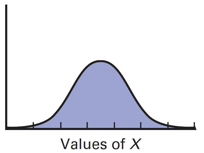
normal distribution

• symmetrical bell-shape

• ranges from negative to positive infinity

• mean determines location

• standard deviation determines spread

• mean = median = mode

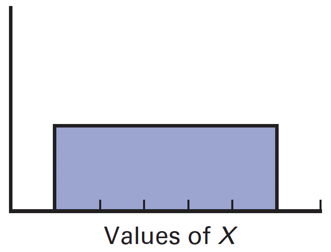
uniform (rectangular) distribution

• all values are equally distributed

• every value is equally likely

• commonly used for completely random events

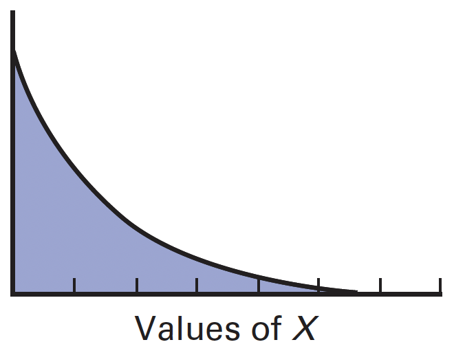
exponential distribution

contains values from zero to positive infinity

right-skewed: mean > median

probability density function

defines the distribution of the values for a continuous variable and can be used as the basis for calculations that determine the probability that a value will be within a certain range

represented by f(X)

standardized normal distribution (Z)

the normal distribution with a mean of 0 and a standard deviation of 1

Z score

tells us how many standard deviations from the mean each value lies