Econ Exam 2

•The classical Keynesian model worked well to explain economic recessions before the.

Great Depression

the AD/LRAS Model =

the Keynesian Model

•Past recessions were based on supply disruptions with items from

POLE decreasing.

•items from POLE decreasing. caused past recessions

oPrices Rise

oGDP Falls

oUnemployment Rises

in the the Great Depression

oCPI Decreased 24%!

•The classical model (AD/LRAS) would not have this:

oCPI Decreased 24%! - •Keynesian model was born.

Keynesian Model:

Short Run Equilibrium

•Key Assumptions: Keynesian Model: Short Run Equilibrium

oSticky or Rigid Prices, §Markets may not be self-regulating.

§Sources of price rigidities (“sticky”)

–Union & other long-term contracts

–Menu costs

–Slow to adjust

§Markets may not be self-regulating., so

Marginal Benefit = Marginal Cost?

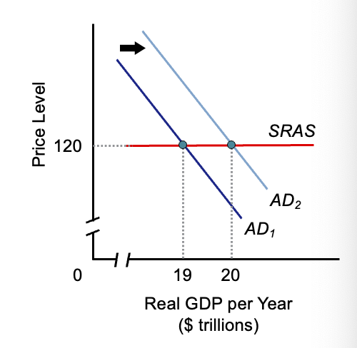
Keynesian Model: Short Run Equilibrium with No

Price Flexibility

Pure Classical Model=

Flexible Prices

Pure Keynesian Model

Rigid Prices

Long-Run View

LRAS determines output.

Short-Run View

Short-Run View

Classical versus Keynesian Models:

Fixed

Classical versus Keynesian Models:

Flexible Prices

Prices _____because, the economy can only create goods and services based on the in the (AD/AS Model

rise in the long run , keys to long run growth.

If there is more demand for goods and services, eventually, firms___because they cannot sustainably continue to create more based on the ___

raise prices , level of POLE.

AD/AS model

•Suppose business investments fall in a nation.  How does this impact the economy in the short run?

a)Prices decrease and real GDP decreases.

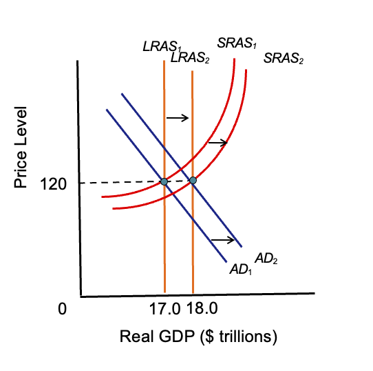
•Increases in Both Aggregate Supply Curves

oShifts Right

oShifts Right in Aggregate Supply Curves

§Discoveries of new raw materials

§Increased competition

§A reduction in international trade barriers

§Fewer regulatory impediments to business

§An increase in labor supplied

§Increased training and education

oShifts Right in Aggregate Supply Curves- §Discoveries of

new raw materials

Shifts Right in Aggregate Supply Curves- §Increased

competition

Shifts Right in Aggregate Supply Curves-§A reduction in

international trade barriers

Shifts Right in Aggregate Supply Curves-§§Fewer___ to business

regulatory impediments

Shifts Right in Aggregate Supply Curves-§An increase in

labor supplied

Shifts Right in Aggregate Supply Curves-§Increased ___ and __

training, education

•Magnitudes

oImportant

oNot Necessarily Same

•M___ Determinants of Long Run & Short Run Aggregate Supply

agnitudes

•Decrease in Short Run Aggregate Supply

oShifts Left

oShifts Left in Short Run Aggregate Supply

§Increased Inflationary Expectations

§Increase in Input Prices

§Increase in Input Prices

–Energy

»Oil, Gas, etc.

–Raw Materials

»Steel, Lumber, etc.

–Wages!

Shifts in ___ Only - Determinants of Long Run & Short Run Aggregate Supply

SRAS

shifts in ___ only

SRAS

•Aggregate Demand Shock

oAny shock that causes the aggregate demand curve to shift inward or outward

•Aggregate Supply Shock

oAny shock that causes the aggregate supply curve to shift inward or outward

•Recessionary Gap means

oGDP < LRAS

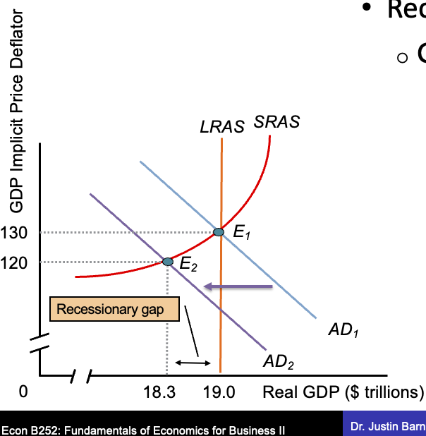
Recessionary Gap

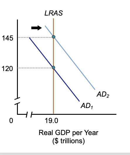
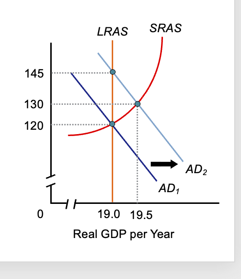
•Suppose exports for a nation increase.  How does this impact the economy in the short run?

a)Prices increase and real GDP increases.

Inflationary gap =

•GDP > LRAS

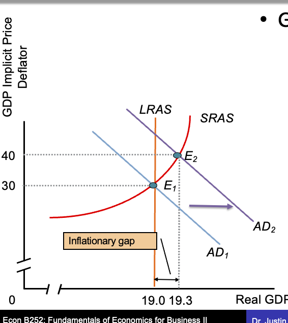
Inflationary Gap

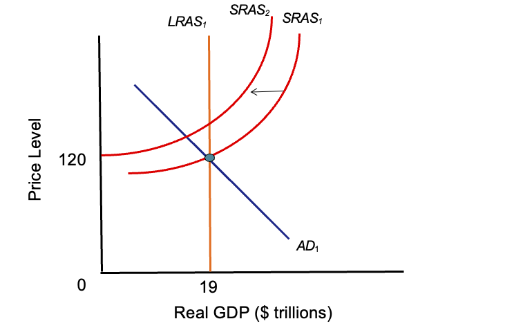
•Suppose wages rise in an economy yet spending does not change.  How does this impact the economy in the short run?

a)Prices increase and real GDP decreases.

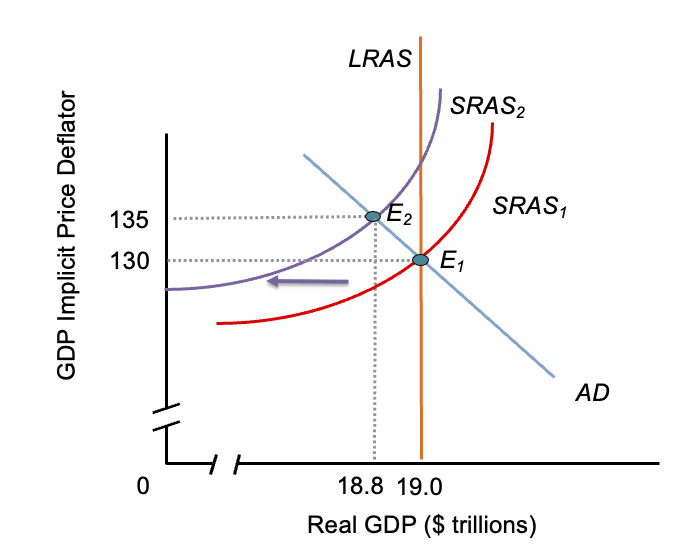
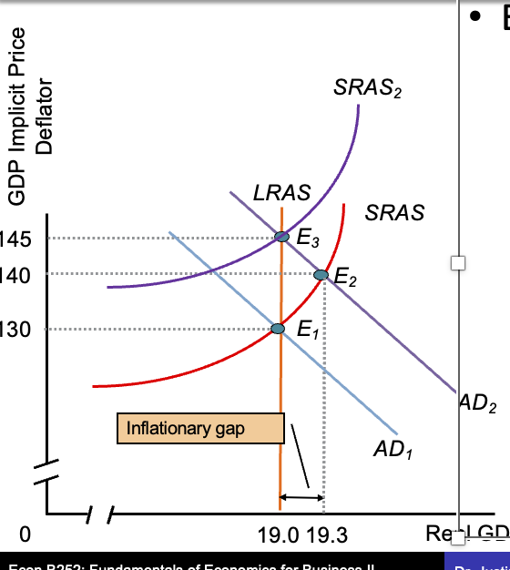
Changes in Short-Run & Long-Run Equilibrium: Two Gaps: Supply Shock

•Economy Correction deflation

“without changes in policy”

“without intervention”

•Economy Correction issues deflation

oInflation Expectations and/or input prices fall.

oSRAS Shifts Right to E₃

oPrices fall more but GDP increases or returns to Potential GDP.

•Economy Correction idea deflation

Return to LRAS

•Economy Correction inflation

oInflation Expectations and/or input prices rise.

oSRAS Shifts Left to E₃

oPrices rise and GDP falls back to potential.

Inflationary gap economy correction

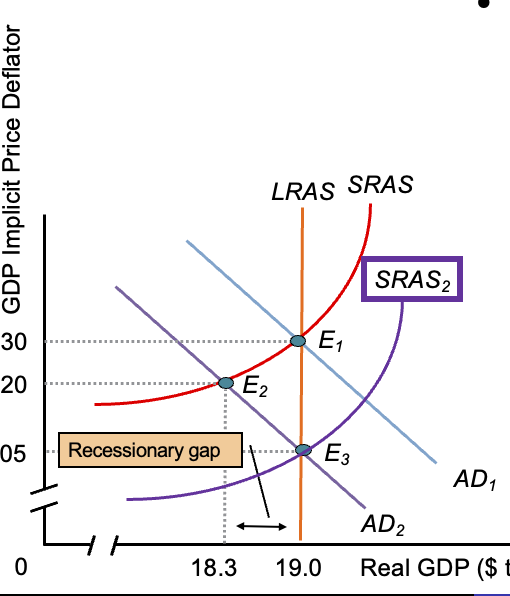
Recessionary gap economy correction

•What would cause the price level to fall and GDP to fall?

a)Aggregate Demand Decreasing

nBetween 2000 and 2001, the price level fell to ___ and real GDP fell to ___

109.7, $9.3 trillion.

nBetween 2000 and 2001, the price level fell to 109.7 and real GDP fell to $9.3 trillion: This result was due to a

leftward shift of the aggregate demand curve.

nBetween 2000 and 2001, the price level fell to 109.7 and real GDP fell to $9.3 trillion.: nDuring this time period, b___ explaining why the ___

business investment in equipment and software (I) fell, price level and real GDP decreased.

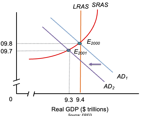
nBetween 2000 and 2001, the price level fell to 109.7 and real GDP fell to $9.3 trillion.

•What would cause the price level to increase and GDP to fall?

a)Aggregate Supply Decreasing

nBetween Q1 2007 and Q4 2008, the price level rose to ___ and real GDP fell to ___

90.8, $15.3 trillion.

nBetween Q1 2007 and Q4 2008, the price level rose to 90.8 and real GDP fell to $15.3 trillion: The result was due to a

leftward shift of the short run aggregate supply curve.

nBetween Q1 2007 and Q4 2008, the price level rose to 90.8 and real GDP fell to $15.3 trillion. Oil prices increased from $71.11 a barrel in July 2007 to ___a barrel in July 2008 explaining why the ___

$145.31 , price level increased, but real GDP fell.

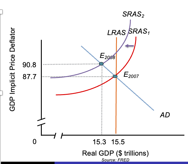
nBetween Q1 2007 and Q4 2008, the price level rose to 90.8 and real GDP fell to $15.3 trillion.

•The simple model can be

misleading

•The simple model can be misleading because

oNo long-run growth (real potential GDP)

oDeflation in model is too common.

•The simple model can be misleading - No

long-run growth (real potential GDP)

•The simple model can be misleading - oDeflation in model is

too common.

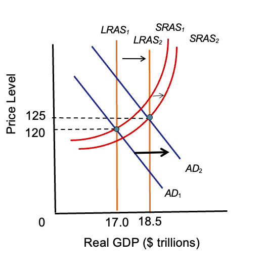
•New Assumptions: Complex Aggregate Demand and Aggregate Supply Model

o§Potential Real GDP Increases

§AD Increases

§SRAS Increases

§Potential Real GDP Increases

§AD Increases

§SRAS Increases in

oMost Years

•LRAS & SRAS Shift Right

oIncreases in POLE

•AD Shifts Right From Increases:

oIncome, Business Spending, Public Goods, International Growth, Money

•Prices and Output

oSRAS & AD in Short Run

§Relative Magnitudes

•AD Increase > SRAS Increase

oInflation

•Economic growth and employment with inflation

•If all three curves increase the same amount

•Economic growth and employment without inflation

•If all three curves increase the same amount

•Economic growth and employment without inflation

•Not very realistic

•If all three curves increase the same amount

•Economic growth and employment without inflation

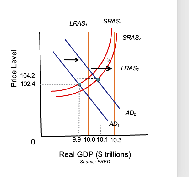
•If AD increases less than LRAS but more than SRAS

•Price level increases (from 102.4 to 104.2):

inflation

•Real GDP increases from $9.9 to $10.1

–But even further below potential

•If AD increases less than LRAS but more than SRAS

•Price level increases (from 102.4 to 104.2): inflation

•Real GDP increases from $9.9 to $10.1

–But even further below potential

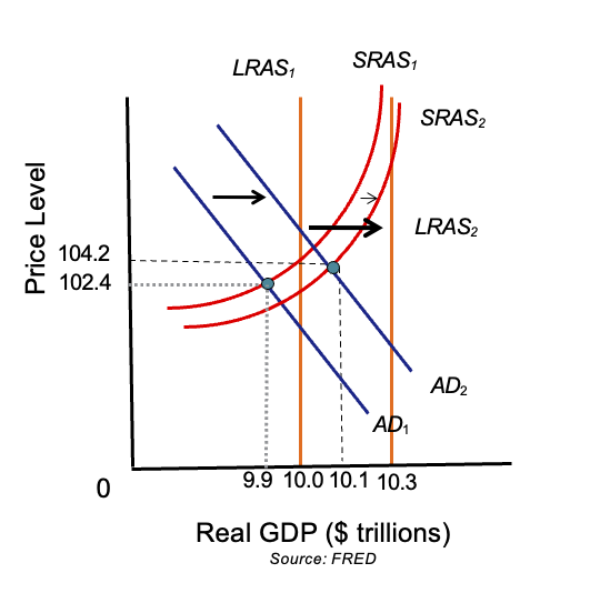
•The dynamic model can illustrate

real world outcomes

•he dynamic model can illustrate real world outcomes

oLRAS & SRAS rise

oAD increases as well but not as much

•The dynamic model can illustrate real world outcomes

oLRAS & SRAS rise

oAD increases as well but not as much

oBigger recessionary gap, but with inflation & an increase in unemployment

Changes in Short-Run & Long-Run Equilibrium: Two Gaps: Recessionary Gap

How does the economy naturally move back to the long run after being in a short run equilibrium that is away from potential GDP?

a)Expected inflation and/or input prices adjust.

oConsumption

§Spending on New Goods and Services

oSaving

§Income Not Used on Consumption

§Income Not Used on Consumption

–Broader than Money in Banks

–Savings at the household level also excludes new housing.

•What is the primary determinant of spending (or saving)?

Disposable Income

Disposable Income

oY_d = Y – T

oY_d = Y – T

§Y is GDP

§Leftover Income After Debts

§Leftover Income After Debts–On the macro level,

»GDP After Taxes

•Disposable Income is ___ or ___

oConsumed, Saved

•Disposable Income

oConsumed or Saved equation

§Y_d = C + S

•Keynes was concerned with changes in

AD.

AD =

C + I + G + NX

•3 ways to look at C + I + G + NX

oTable Form (Less Focus)

oGraph Form (Less Focus)

oAlgebraic Form

•Consumption Function is

orelationship between consumption and disposable income

•Consumption Function equation

§Spending = Slope*(Disposable Income) + Constant

•Marginal Propensity to Consume (MPC)

oThe ratio of the change in consumption
 to the change in disposable income

•Marginal Propensity to Consume (MPC) changes are

differences.