psyc 2100wq exam 1
1/102
Earn XP
Description and Tags
exam 1 lecture notes
Name | Mastery | Learn | Test | Matching | Spaced | Call with Kai |
|---|
No analytics yet
Send a link to your students to track their progress
103 Terms
empirical science
observation based and numerically observed science
construct
thing to be observed
must be defined before numerical observation
“what” is observed
operationalization
identification of measurement procedure for measuring external behavior — then uses resulting measurements as definition and measure of a hypothetical construct
“how” something is observed
variable
characteristic or condition that changes or has different values for different individuals
determined and declared after observation
cannot be considered a variable unless observed to show variation
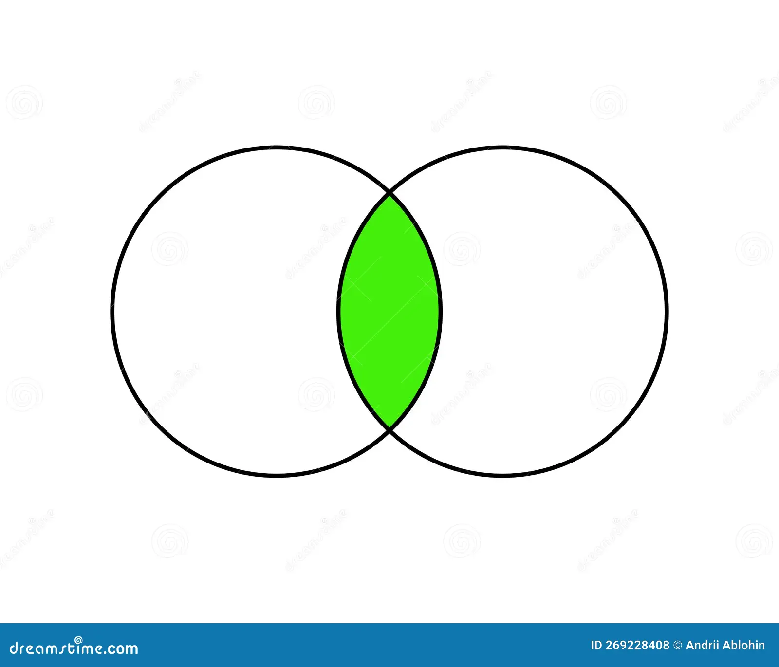
covariation
the variation of one thing - shown to be related to the variation of another thing
simple covariation
non-ordered — absence of specified order in reference to 2 variables that vary together
ordered covariation
order of covariation is specified
shows causality
done only by manipulation and shown IV/DV relationship — experimental
data
numerically recorded observations
Hypothesis
formal statement of what a researcher believes is true
declared in a written/verbal statement to the public
experimental group
receives treatment/manipulation
control group
does not receive treatment/manipulation
causality
assume variation that occurs due to or as a result of cause and effect
1-1 causality
for every cause there is an effect
chain of cause and effect (cause and effect links)
C1—> E1 (becomes c2) —>E2 etc.
simple covariation diagram
V1 ←→V2
ordered covariation diagram
V1 →V2 or V1 ←V2
mutually exclusive, only 1 can occur at one time
confound variable/third variable
only determined under ordered covariation
3rd variable that may be the cause of both or either V1 or V2
statistic
set of mathematical procedures for organizing, summarizing and interpreting information and numerically numbered observations
percent
0-100
frequency
0-infinity (highest number possible
proportion
0 -1.00
descriptive statistics
used to describe the sample measured
inferential statistics
used to draw inferences/predictions about the population (can be applied to generalize)
Population
unspecified N number of individuals for which we have numeric observations
only exists bc theorized to exist
sample
specified/known number of individuals from population
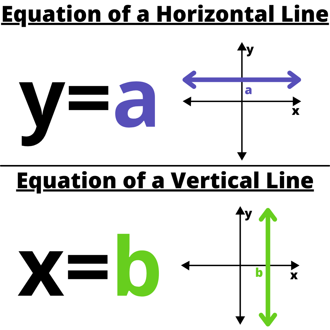
skewed
line drawn over distribution is not a bell shape
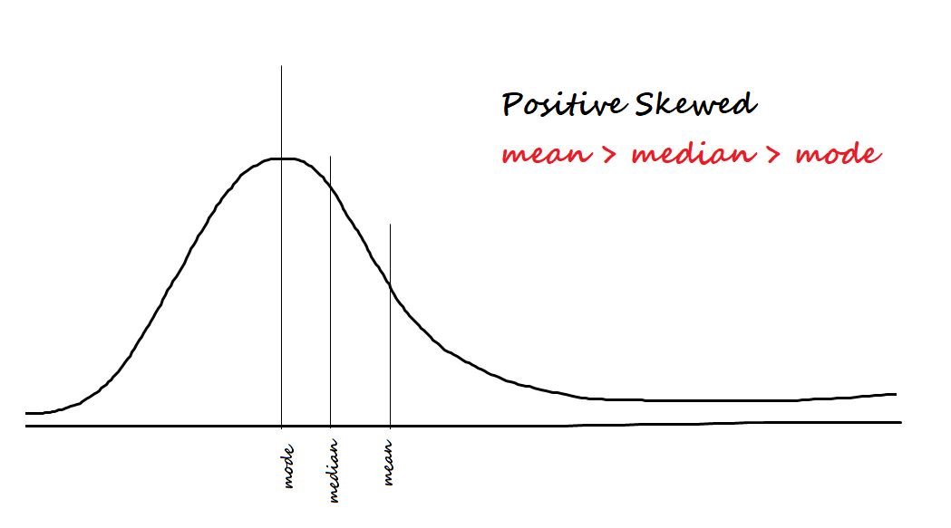
positive skewed
tail falls on positive side (the right) and high frequency on the left
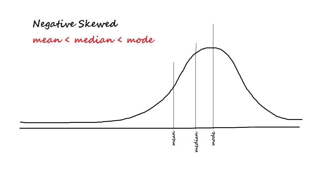
negative skewed
tail falls on the negative side (the left) and high frequency of scores on the right
frequency distribution
visual of low to high scores — all scores fall under the line
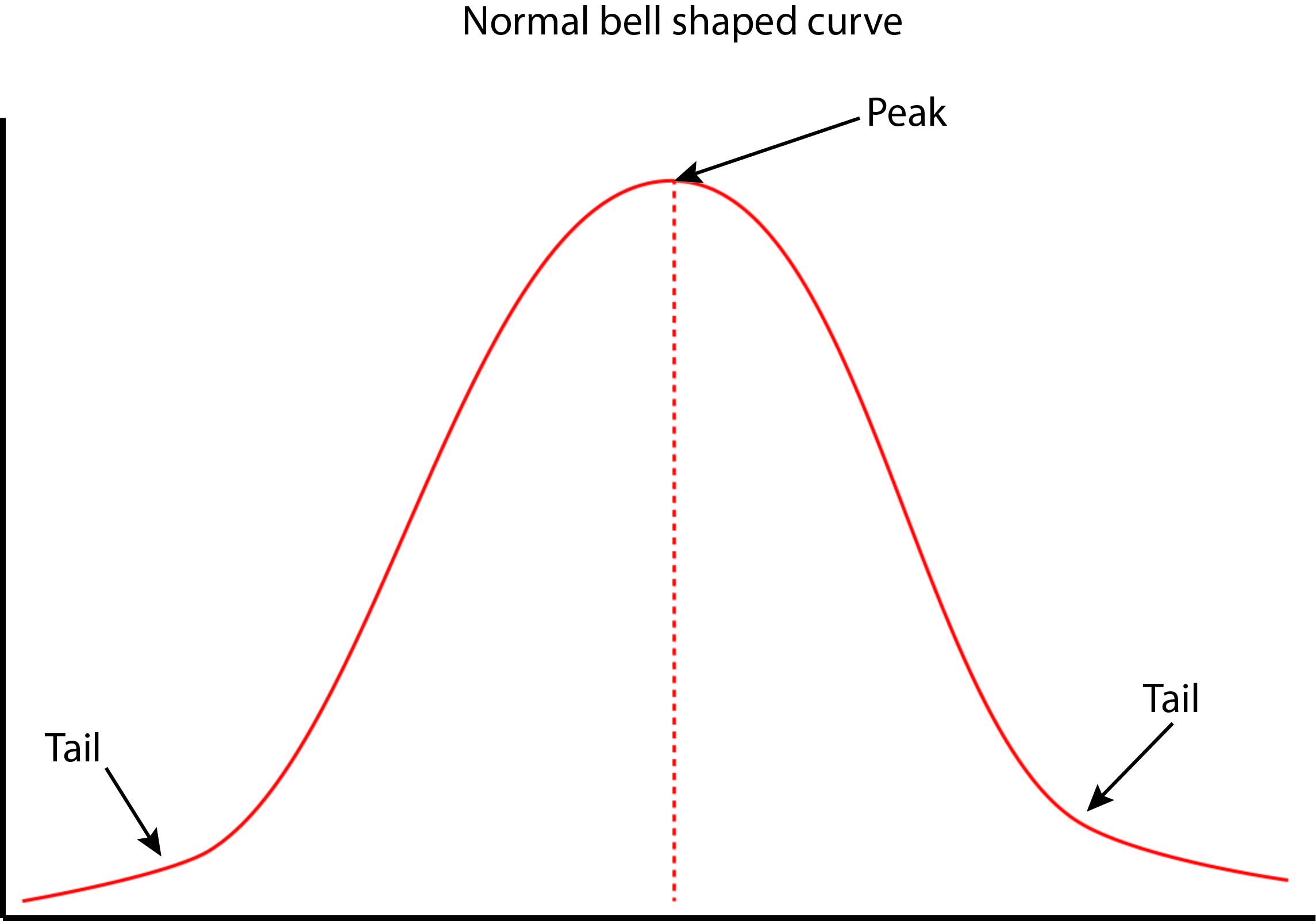
bell shaped distribution
scores in the middle show highest frequency then trail off along both sides
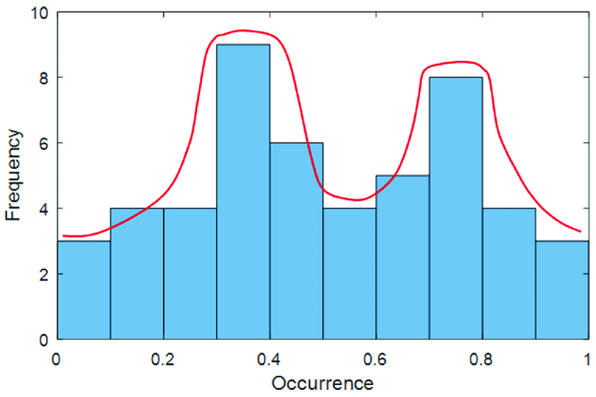
bimodal distribution
contains 2 peaks
best when use 2 modes to describe this data
population parameter
value that describes a population, usually derived from measurements from individuals in the population
sample statistic
value that describes a sample
mean for population (parameter)
μx=∑x/∞
we can theorize this exists but cannot actually numerically represent it
Mean for sample (statistic)
x̄= ∑x/N
can be used as an inference about the population
median (Md)
used when there is skewed distribution or presence of outliers
the number that falls directly in the center of the distribution of scores
mode(Mo)
score in distribution that occurs with the highest frequency
done with bimodal data or nominal data
central tendency
representation of where scores tend to show highest frequency
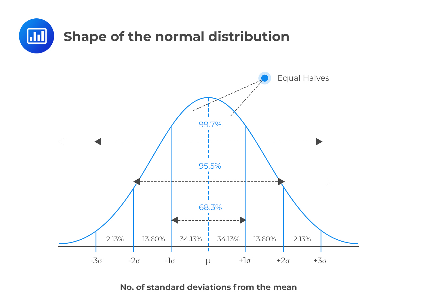
normal distribution
bell shaped curve
mean, median and mode are all the same number
show symmetry — proportion of scores on both sides of the central tendencies is .50
standard deviation
indicates variation of scores in a distribution
amount on average the scores deviate from the mean
high standard deviation
more on average that scores deviate from the mean
low standard deviation
less on average that scores deviate from the mean (clustered together)
standard deviation equation (for sample)
S= √ (∑(x-x̄)2/n-1)
Standard deviation equation (for population)
S= √ (∑(x-x̄)2/N)
variance equation
Variance = (∑(x-x̄)2/n) NO SQUARE ROOT)
what does the equation for standard deviation mean
the square root of the sum of squared deviations (or deviations squared) over the number summed
normal distribution frequency
from -1s to 1s = .683
from -2s to 2s = .955
from -3s to 3s =.997
frequency distribution table
x | f | % | P |
1 (female) | 30 | 60% | .60 |
0 (male) | 20 | 40% | .40 |
simple covariation hypothesis example
self esteem is related to academic success
ordered covariation hypothesis example
self esteem training (IV) leads to academic success (DV)
design of a study
must be indicated before data is collected
determines how the data is to be collected (procedures)
types of designs
experimental versus non-experimental
chosen based off of whether hypothesis is ordered or simple
case study
non-experimental design
observes 1 individual
used often when permission to observe someone is difficult to obtain
naturalistic observation
setting in which variation naturally occurs + can be observed
ex. observation of birds
trial
indicates and specifies where and when the data are going to be collected and how many trials will be done
lab environment
can control variation of everything except for the one thing you are manipulating to vary
experimental design
ordered covariation is used
one variable is manipulated while others are observed in relation to that manipulated variable
shows IV, DV relationship
can determine cause and effect
ex. mechanical birds head bop study
skepticism
the suggestion of doubt about a claim of what is true (a knowledge claim)
always present in science bc knowledge claims are never absolute
threat to validity of study (rectify by adjusting or building a design to fit)
validity of design
basis by which a claim is made sufficient and reasonable
is the design of the study sufficient for providing empirical basis of knowledge claim
external validity
does the IV-DV relationship as observed in the study generalize beyond the study to other settings, people or other points in time
ex. bird study did not address female female interactions — perhaps specific to “like-gender“ interactions not just male-male interactions)
internal validity
did the IV really cause variation in the DV or is the variation due to something else
ex. adding control group to SE study bc possibly AS affected by attention given not just the actual content of SE training — give control group 90 minutes of attention unrelated to SE
measurement
aka measure, scale, test
used to assign numbers to observations
used to operationalize how numbers are assigned to operations — record numeric operations
psychometrics
generation of criteria to evaluate goodness of a measure
Reliability (in reference to measurement and in reference to scores yielded)
consistency — do the scores yielded by the scale show consistency
over time, over different measures of scale or over responses of individuals to the measures
validity (in reference to measures and scores yielded by measures)
accuracy — do the scores yielded by the scale give a correct representations of the “low-high” variation of the variable of interest
covariation
can be used to indicate consistency /reliability
pearson product moment correlation coefficient
measures the degree and direction of the linear relationship between 2 variables
=r
done on a -1 to 1 scale
r=.00
the grounding point
absence of covariation in data
allows for show of HOW MUCH covariation there is
1,2,3
1= departure from 0 shows there is covariation present in the data
2= if more than 0 — there is positive covariation, if less than 0 — there is a negative correlation
3= HOW MUCH positive or negative covariation is present
test-retest design (reliability)
can examine consistency of scores over time
ex. test same individuals at 2 separate times, (t1 and t2) — if scores show consistency across time — the measure is reliable
equivalent/parallel forms design (reliability)
consistency of scores across different scaling formats
ex. individuals self-report SE on 5 item scale ranking system + same individuals show the same/consistency in scores when done in interview format with a scorer of the same 5 item ranked scale.
inter-item reliability design (internal consistency design)
consistency of responses to items on the scale
ex. amount on average of consistency of covariation in respect to all possible pairs of items
use of inter-item correlation matrix
r̄
the average of coefficients
cronbach’s alpha is roughly equal to this
r̄=∑x/N
correlation matrix
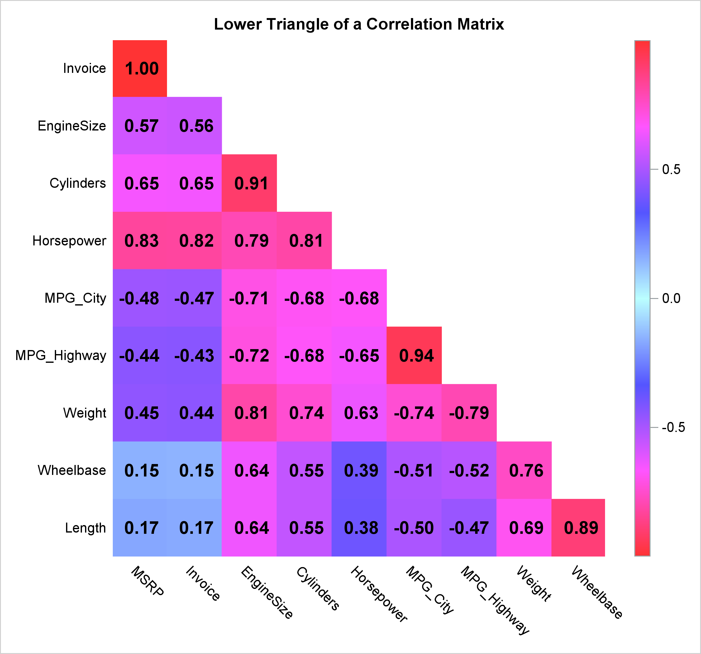
scores yielded by scale
provides a correct representation of low-high variation of variable of interest
predictive criterion-related design (validity)
accuracy of scores yielded by scale showing a predictor —> criterion relationship
ex. self estreem measured at time one predicts academic success measured at time two — measured at 2 different times to see if SE is a predictor for AS (criterion)
coupling hypothesis
used to show multiple hypotheses
H1 — SE is related to AS
H2 — SE at T1 predicts AS at T2
convergent-discriminant validity design
convergent — the ones you think do show covariation and relate
discriminant— something that could be related but when shows no covariation between 2 other items shows accuracy of measuring the thing your’re intending to measure and not something else
ex. H1 — SE is related to AS but is not related to optimism — convergent coefficient (SE + AS show r=.60) versus discriminant coefficient (SE + OPT show r= .05)
covariance
used to derive correlation coefficient (r)
the average of how deviations scores of x relate to deviation scores of Y
covariance equation
COV = ∑(x-x̄)(y-ȳ)/n-1
coefficient derived from covariance equation
r= COVx(y)/(Sdx)(Sdy)
why do we use pearson’s coefficient
because of the underlying metric of -1 to 1 — allows indication of how much correlation/covariation there is
what does pearson’s correlation do
indicates linear relationsip amount (from a straight line) and the slope of that line
linear
in reference to a straight line
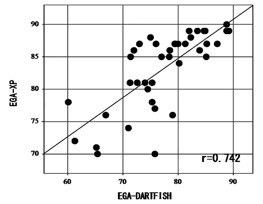
bivariate scatter plot
two variables measured and plotted in a scatterplot
Line of best fit
given scatter plot of all points of individuals — straight line closest to all possible points that is better than any other line
undefined/ideterminate
coefficient does not exist because one variable does not have variation — need variation for both in order to have a coefficent
class rule !
before interpretting a coefficient — plot the data
moderate positive correlation
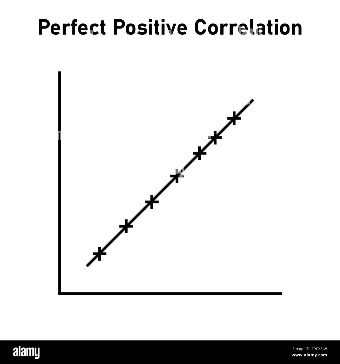
perfect positive correlation
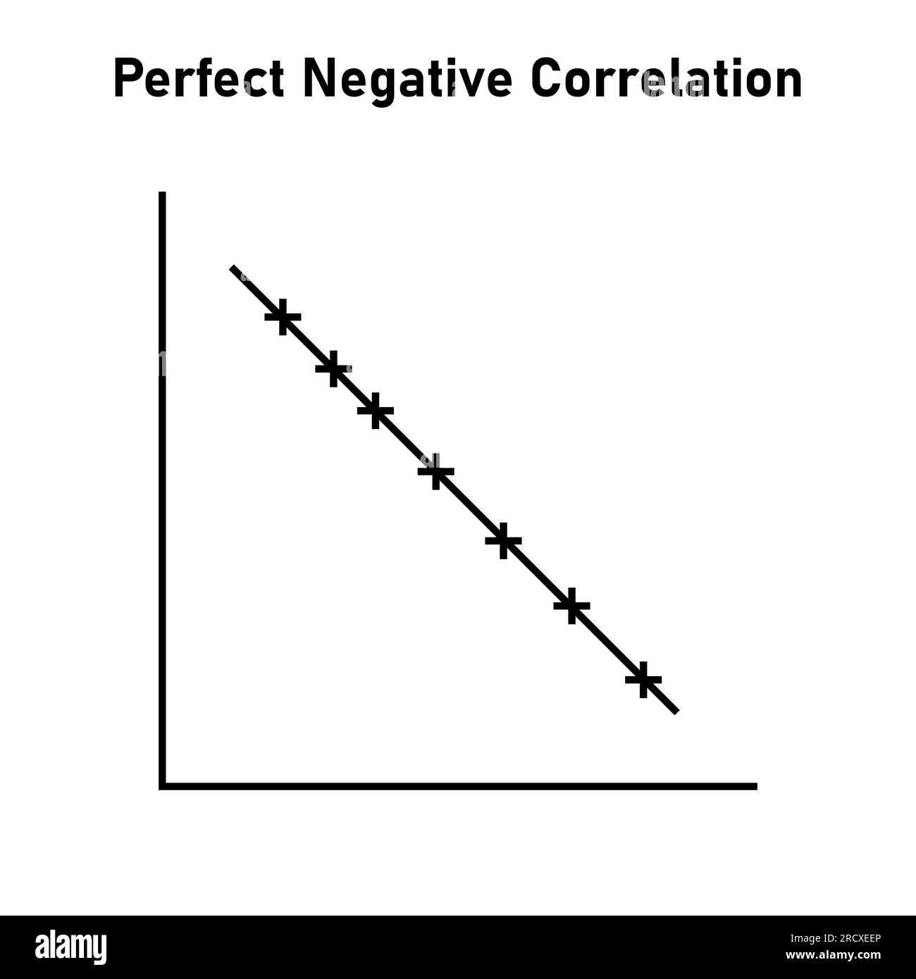
perfect negative correlation
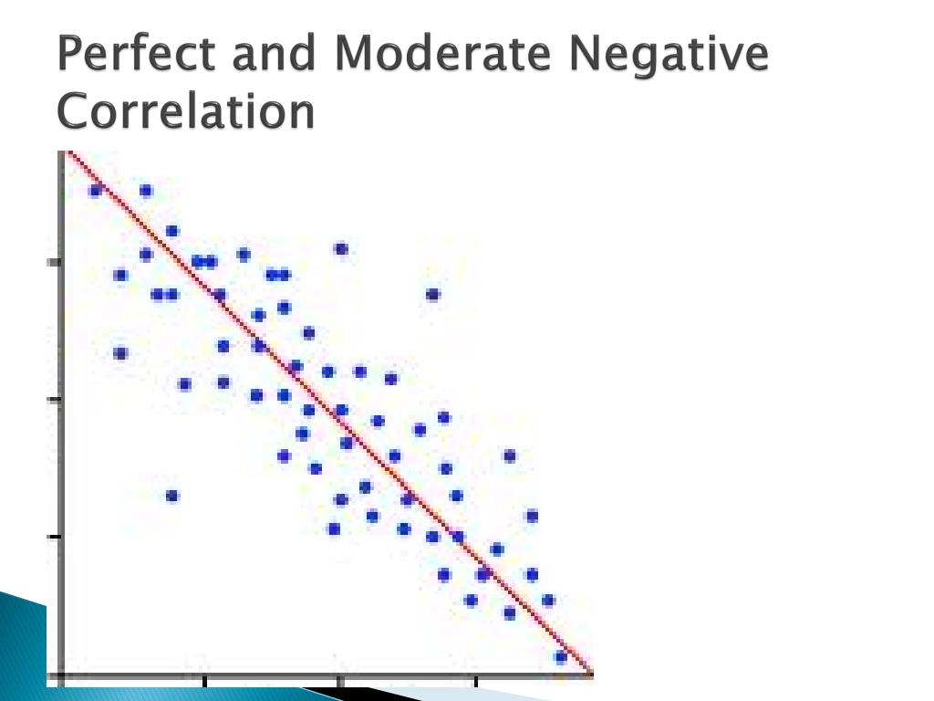
moderate negative correlation
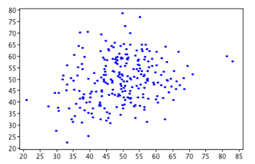
circular no correlation
undefined correlation
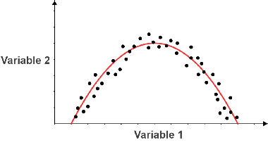
curvilinear relationship
shows no correlation for pearson’s correlation
r2
proportion of shared variation
to what extent does the variation in x relate to the variation in y
allows for widening audience by allowing % of shared variation to be determined
indicates proportion of variation in x that has been observed in variation of y
problems of interpretation in coefficient
range restriction, selection effect and small sample — all give only part of the possible points on a scatter plot
artifact
something that appears to be true but is not
small proportion of shared variation
r= .25, r2= .06 = 6% of variation in x has been observed with variation in y
moderate proportion of shared variation
r=.50, r2= .25 = 25% of shared variation