Statistics 2 Lecture 12

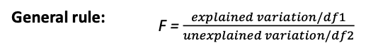
F-tests: Variation

• Numerator: Explained variation

  • Global F-test: Variation explained by model (RSS)

  • Model-comparison F-test: Variation uniquely explained by extra parameters complete model (𝑆𝑆𝐸𝑟 –𝑆𝑆𝐸𝑐)

  • Test for one effect (F)AN(C)OVA: Variation uniquely explained by factor or effect

• Denominator: Unexplained variation

  • Global F-test: Residual sum of squares model (SSE)

  • Model comparison F-test: Unexplained variation complete model (𝑆𝑆𝐸𝑐)

  • Test for one effect (F)AN(C)OVA: Residual sum of squares model

F-test: Degrees of freedom

• df1: How many parameters used to explain variation in numerator?

  • Global F-test: Number of b-coefficients in model (k)

  • Model-comparison F-test : Difference in #b-coefficients complete and reduced model (𝑑𝑓c – 𝑑𝑓r )

  • Test for one effect (F)AN(C)OVA: Suppose we’d use GLM: How many dummies (and thus #b-coefficients) needed to model this specific effect?

    • E.g.,. ANOVA: 𝑔 − 1

• df2: Freedom left after estimating entire model.

  • In regression (with dummies): N – (k + 1)

  • Modelvergelijking F-toets: dfc = N – (k + 1) complete model

  • In (F)AN(C)OVA: N – (k + 1) When you would use regression with dummies.

Before we draw conclusions

We should check, if

• There are gross violations of the model’s assumptions

• There are any influential observations that may (potentially incorrectly) influence our conclusions

Concerning assumptions, we can differentiate between

• Designeffects [methodological check]:

  • Random sample (representative and independent observations) - crucial

• Assumptions about the association and distribution of the data:

  • True regression function has the form as used in the model (e.g., linear) (Functional form) - crucial

  • Conditional distribution of y is normal (normality of residuals) - less important as N increases

  • Conditional variation around the regression equation is constant for all x (homoscedasticity of residuals) - quite robust, but other model/estimation procedures may be more suitable

Check model assumptions GLM

• States that the prediction errors for all values of x (𝜖𝑖):

  • Are normally distributed

  • Around an average value of 0

  • With equal (homogeneous) variation 𝜎

• And therefore do not show any structure.

• Can be inspected using plots of the [standardized] residuals!

Assumptions for ANOVA

• In case of a categorical predictor:

  • All values of x: all levels of the factor (all groups)

  • Conditional variance: Within-group variation

• We thus need:

  • Normal distribution in each group

    • Check histograms within groups

  • Equal variation across the different groups

    • Use Levene’s test + SDs within groups

• ANCOVA: Also homogeneous regression slopes

  • No interaction-effect between cat and quant predictor

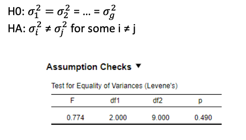
Levene’s test

• Tests the assumption of homogeneous variance across groups

• Test is quite sensitive for sample size.

  • For large samples, a small difference in 𝜎’s cam yield a significant result.

  • For small samples, a large difference in 𝜎’s may not yield a significant result.

• Reminder:

  • ANOVA is quite robust concerning homogeneity

  • We check for gross violations of the assumptions.

• Thus also inspect the degree to which 𝜎’s differ

• Rule of thumb: Largest SD max 2x smallest SD.

• Conclusion example: We cannot reject H0! We have no evidence against the assumption of homogeneous variance across groups.

Extra Assumption ANCOVA

• Suppose we see the following pattern in a scatter plot

  • Due to interaction-effects between predictors (Software and Stat1Grade)

• In case of interaction between factor and control variable, it is not meaningful to compare adjusted means.

  • Because: [adjusted] difference between grades of R and JASP students depends on the value of Stat1grade!

• Therefore extra Assumption for ANCOVA: Homogeneous regression slopes

  • Association between control variable and y should be the same for all groups (i.e., parallel lines; no interaction)

  • Thus: Always test for interaction-effects between factor and control variable!

  • When interaction: compare group means at multiple levels of X

Influential observations

• There may be individual observations that deviate strongly from the general trend. We call such observation regression [or multivariate] outliers.

• These can potentially influence our conclusions.

• Not every outlier is influential. Depends on two aspects:

• Degree to which an observation’s y score deviates from the trend (𝒚 predicted)

  • Summarized as the studentized [standardized] residual

  • Studentized residuals > 3 are potential outliers and should be checked.

  • Perhaps it’s a measurement error, type or from a participant that does not belong in the sample.

• How the observation’s predictor values (x) deviate from the mean (𝑥 mean)

  • Summarized as the leverage

  • The stronger the deviation from the average x, the stronger the leverage

  • The smaller the sample, the higher the leverage

• The higher the leverage the stronger the potential influence of an observation in determining the regression equation for 𝑦 (predcited) and 𝑅2!

• Useful to check if the fit of the model (R2) or the regression parameters in which you’re interested (b) are strongly influenced by such observations.

Relevant measures to identify influential outliners

• DFBETA’s: Summarizes for each observation per b-coefficients: Effect on the parameter estimates if you would remove the observation from the model

• DFFIT en Cook’s D: Summarizes per observation: Effect on the fit of the model (i.e., SS and 𝑅2)

• Therefore: Check for standardized residuals with absolute values > 3

• Present?

  • Check if these are simply mistakes in the data

  • Check the influence using DFBETA and DFFIT or Cook’s distance (e.g.,. Using 4/n or > 1)!

Models for non-linearity

• Sometimes, we see (or expect) a non-linear association between x and y

• Non-linearity: The association between x and y changes, when x increases Example: Association between stress and performance (Yerkes-Dodson Law):

  • Performance increases with arousal (stress)

  • Up to a certain point

  • To much stress leads to a decline in performance

• Solution: Include a quadratic term of x in regression model

Models for dependent y

• Sometimes, we know prior to our analyses that our assumptions of GLM or (F)AN(C)OVA are violated.

• Dependent samples: Repeated measures or clustered observations

Example repeated measures

• Same participants are repeatedly tested in different conditions

• Example: Every student makes assignment in both R, JASP and SPSS.

• There are differences in results within persons and between persons

• Should not use ANOVA: Independence of residuals is violated

• Solution: Repeated measures ANOVA

  • Levels of Factor [categorical predictor] differ within persons

    (e.g.,. T1, T2, T3, or drug 1, drug 2, drug 3)

  • Modelling within- and between-person effects

Example clustering

• Research on association hours study and test scores

• Data includes multiple students per school

• Students of same school have same experiences, educational quality, etc.

• Their observations are thus dependent: Test scores within schools are likely more similar than test scores between schools.

• Independence of residuals is violated

• Solution: Linear mixed model (c.q. multilevel model; part of Generalized linear model)

  • Fixed effects (a and b’s as in regression)

  • Random effects (a and b’s can vary across clusters/persons)

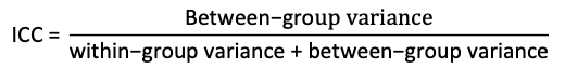
  • Intraclass correlation coefficients as measure of dependency

  • Source of dependence must be known to compute ICC and use linear mixed model.

Models for categorical y

• Diagnoses

  • Presence of mental disorder (yes/no)

  • Type of anxiety disorder (generalized, panic, fobia)

• Attachment style

  • Safe, anxious, avoidant or disorganized

• Education flow

  • Degree obtained (yes/no)

  • Educational level (vocational, professional, academic)

• Problem: No linear association between x and y. Residuals not normal and not homogeneous distributed for all x.

• Solution: logistic regression (part of Generalized linear model)

  • Predicts function of y instead of y itself (log)

  • We inspect odds or probabilities of a specific outcome, instead of (changes) in predicted y.

  • Odds ratio as effect size