Statistics Lecture 3

Hypotheses, study characteristics and variables

• Cross-sectional study across randomly selected schools in the Netherlands

• Three quantitative variables:

  • y: Response variable, also called outcome (in this case academic performance)

  • x1 and x2: Explanatory variables, also named predictor (in this case class size and percentage of free meals as an indicator of socio-economic background)

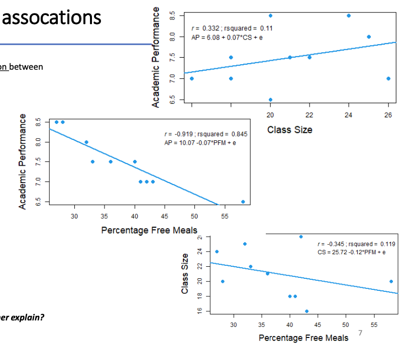
Describing the bivariate associations

• Scatter plots show the bivariate association between all possible pairs of variables:

• Academic performance and class size:

  • → Positive association

  • → CS explained 11% of the variation in AP

• Academic performance and percentage free meals:

  • → Negative association

  • → PFM explained 85% of the variation in AP

• Class size and percentage free meals:

  • → Negative association

  • → PFM explained 12% of the variation in CS

• Q: How much variation in AP will PFM and CS together explain?

• Not simply the sum of 85% and 11%: they are confounded (i.e., CS shares 12% of its variation with PFM)

• → We need a multiple regression model

The multiple regression model

• We include multiple predictors of our outcome variable y.

• 𝑦 =𝑎+𝑏1∗𝑥1+𝑏2∗𝑥2+⋯+𝑏𝑘∗𝑥𝑘+𝑒

• a is still the intercept: Expected y when all x are 0

• b’s are the regression slopes for each predictor variable: b1 for x1; b2 for x2; ... ; 𝑏𝑘 for 𝑏𝑘

• The meaning of the 𝒃’s differs from the meaning of b in simple regression!!

• → Statistical control: effects of all other x on both 𝑥𝑖 and y are eliminated!

• For example:

• AP = a + b1 CS + b2 PFM + e

• a = the expected AP for schools with CS and PFM = 0

• b1 models the association between CS and AP: →After controlling for the effect of PFM on both CS and AP

• b2 models the association between PFM and AP, but: →After controlling for the effect of CS on both PFM and AP.

Controlling for other predictors

• b’s in the multiple regression model are about the association between x and y when we eliminated the effect of all other predictors in the model on both x and y

• What differences across individuals do we observe in x and y after eliminating the effect of all other x?

• Can these residual differences in x explain the residual differences in y?

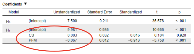
Coefficients b in a multiple regression model

• AP = a + b1*CS+ b2*PFM + e = 9.981 + 0.003*CS – 0.067*PFM + e

• b1 models the association between CS and AP:

  • → After controlling for the effect of PFM on both CS and AP.

  • →That is, the association between the residuals of AP = a + b*PFM + e = 0.003

• and the residuals of CS = a + b*PFM + e

• Same holds for b2: b2 models the association between PFM and AP, but:

  • →After controlling for the effect of CS on both PFM and AP.

  • →That is, the association between the residuals of AP = a + b*CS + e and the residuals of PFM = a + b*CS + e = -0.067

Interpretations of coefficients b in multiple regression

• The expected change in y for a one-unit increase in predictor x while statistically controlling for all other predictors in the model.

• The expected change in y for a one-unit increase in predictor x when all other predictors are kept constant.

• The effect of predictor x on outcome y among subjects with the same score on the other predictors.

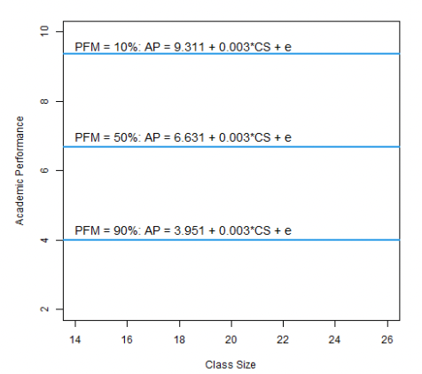
• For example, b1 = 0.003:

  • Academic performance is expected to increase by 0.003 when class size increases with 1 student and the percentage of students with free meals is kept constant.

  • Among schools with the same percentage of students with free meals, we expect the performance to be 0.003 higher for each additional student in a class.

  • → Given this model, intercepts (a) differ for varying levels of PFM, but the ‘partial effect’ of CS remains the same (0.003).

  • → That is because we statistically controlled for the effect of PFM. Keeping PFM stable at ‘some’ level, the effect of CS on AP is 0.003!

Summary: Regression coefficients a, b1 and b2

• Linear multiple regression model: 𝑦 = 𝑎 + 𝑏1𝑥1 + 𝑏2𝑥2 + 𝑒

• Predictor variables: x1 and x2 Coefficients:

• 𝑎: y-intercept: Expected Y value when all x are 0

• 𝑏1 and 𝑏2: slopes [partial effect] for x1 and x2

  • 𝑏1: Expected change in y for a one-unit increase in x1 when all other x’s are kept constant.

  • 𝑏2: Expected change in y for a one-unit increase in x2 when all other x’s are kept constant.

• Can be extended with any number of predictor variables (k)

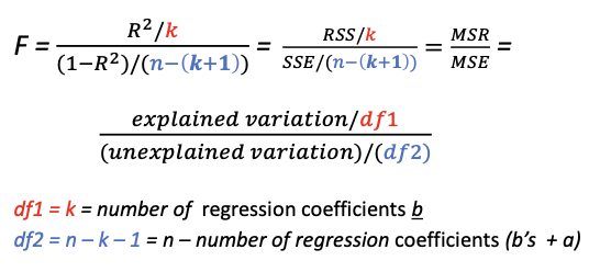
Hypothesis testing in multiple regression: The F-test for R2

• Multiple null-hypothesis significant tests exist for models that include multiple predictors

• Global F-test: Do the predictor variables collectively explain variation in the outcome variable?

• H0:𝜷𝟏 =𝜷𝟐 =⋯=𝜷𝒌 = 𝟎
  →None of the predictors x is associated with y →Same as saying, the population 𝑅2 = 0

• Ha: at least one 𝜷𝒊 ≠ 𝟎
  →At least one of the predictors x is associated with y →Same as saying, the population 𝑅2 > 0

• MSR: How much variation is explained per predictor in the model?

• MSE: How much variation can on average be explained by each additional predictor that we, given the sample size, could potentially add to the model.

• F = ratio of the two. When F > 1: the predictor(s) explain more variation in y than is expected from any randomly selected additional predictor.

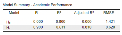
Results of the Linear Regression Model: Model Summary

• 𝑅2 is .811

• Calculated as SSR/TSS = 653.26/805.844
  o Thus: About 81% of the variation in academic performance across schools is explained by class size and the percentage of free meals in a school.

• → A large percentage!

Results of the Linear Regression Model: ANOVA table

• RSS (Regression sums of squares) = 653.26

  • Variation in y that is explained by the model.

  • df1 = k = 2 →(b1 and b2)

  • Thus: MSR = 653.26 /2 = 326.63

• SSE (Sums of squared errors [residuals]) = 152.58

  • Variation in y that is not explained by the model.

  • df2 = N – k – 1 = 400 – 2 – 1 = 397

  • Thus: MSE = 152.58 / 397 = 0.38

• TSS (Total sum of squares) = 805.84 → (same as for the simple regression: The regression model does not change the observed variation in y)

• The F-statistic for the model is 849.87

  • Calculated as MSR / MSE = 326.63 / 0.38

  • With df1 = 2 and df2 = 397, this yields p < .001

  • The model—including linear effects for class size and percentage of free meals—thus explains a significant portion of variation in academic performance.

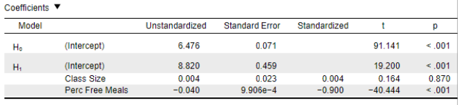
Results of the Linear Regression Model: Coefficient table

• The constant (intercept, a) is 8.820

  • This is the predicted academic performance in schools with a class size (x1) and percentage of students with free meals (x2) of 0.

• The coefficient for ClassSize (b1) is 0.004 with p = .870 and b1* = 0.004

  • The coefficient is positive but non-significant and negligible.

  • Thus, after statistically controlling for the percentage of free meals in a school, we find no evidence for an association between class size and academic performance.

  • → Note the difference compared to last week’s simple regression, when we found b = 0.18, SE = 0.05, t (398) = 3.54, p < .001!

  • → Thus, CS and AP are positively related, but not after controlling for PFM.

• The coefficient for Perc Free Meals (b2) is -0.040 with p < .001 and b2* = -0.900.

  • The coefficient is negative, significant, and considered large.

  • Thus, after statistically controlling for class size, we find evidence for a strong association between the percentage free meals in a school and academic performance.

Conclusion

• The model—including linear effects for class size and percentage of free meals—is significant. Together, these predictors explains 81% of the variation in academic performance, which is considered large explanatory power.

• Class size and academic performance are positively related, but when we statistical controlling for differences in the percentage of free meals in a school, we find no evidence for an association between class size and academic performance.

• Also: The percentage free meals in a school is strongly and positively associated with academic performance, even after controlling for differences in class size.