Chapter 4 - National Income and Price Determination
1/69
Earn XP
Description and Tags
Name | Mastery | Learn | Test | Matching | Spaced |
|---|
No study sessions yet.
70 Terms
Marginal Propensity to Consume (MPC)
The income in consumer spending when disposable income increases by $1.
Marginal Propensity to Save (MPS)
1 - MPC. The increase in household savings when disposable income rises by $1.
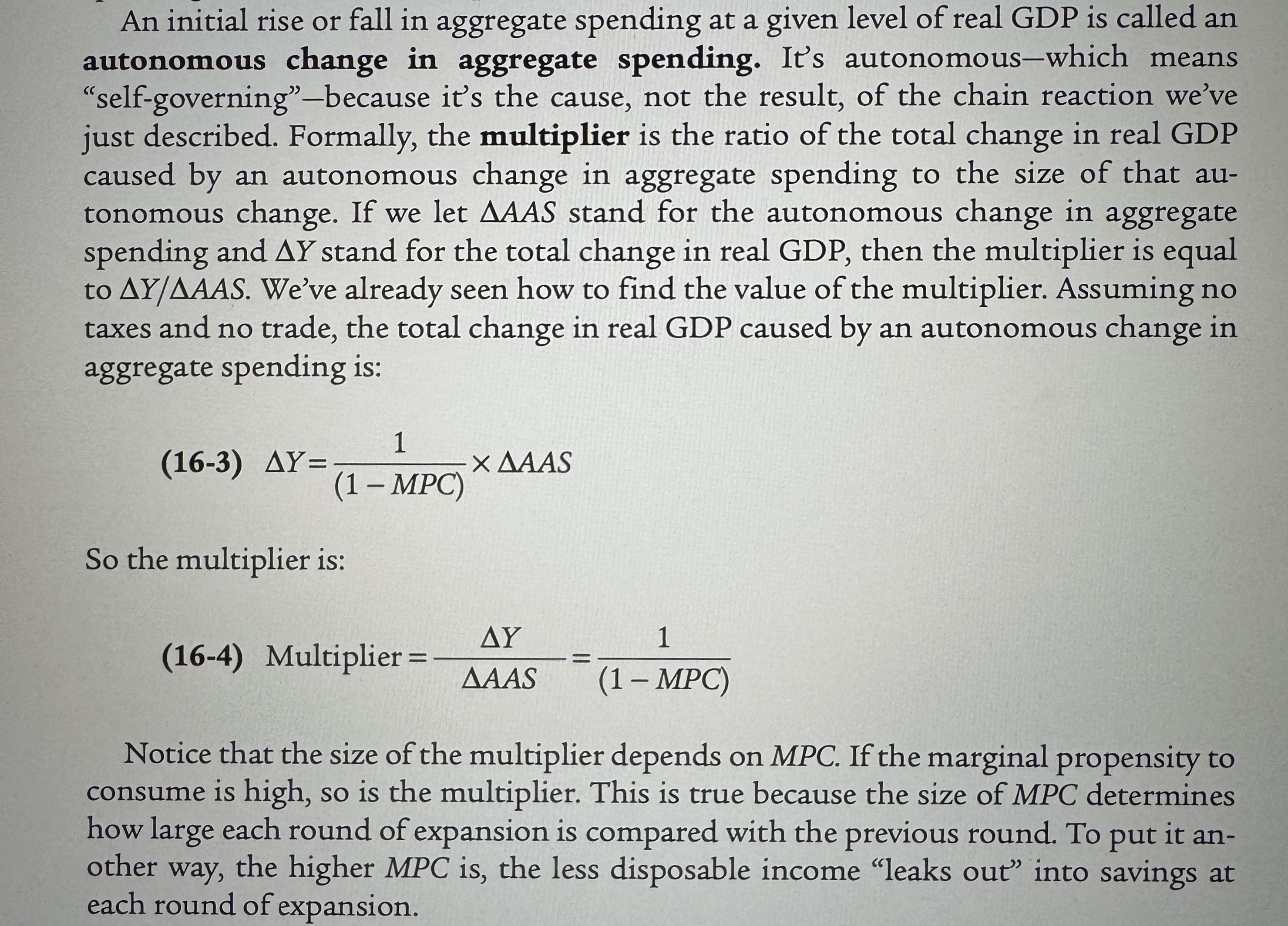
Autonomous Changes in Aggregate Spending
An initial rise or fall in aggregate spending that is the cause, not the result, of a series of income and spending changes
The Multiplier
The ratio of the total change in real GDP caused by an autonomous change in aggregate spending to the size of that autonomous change.
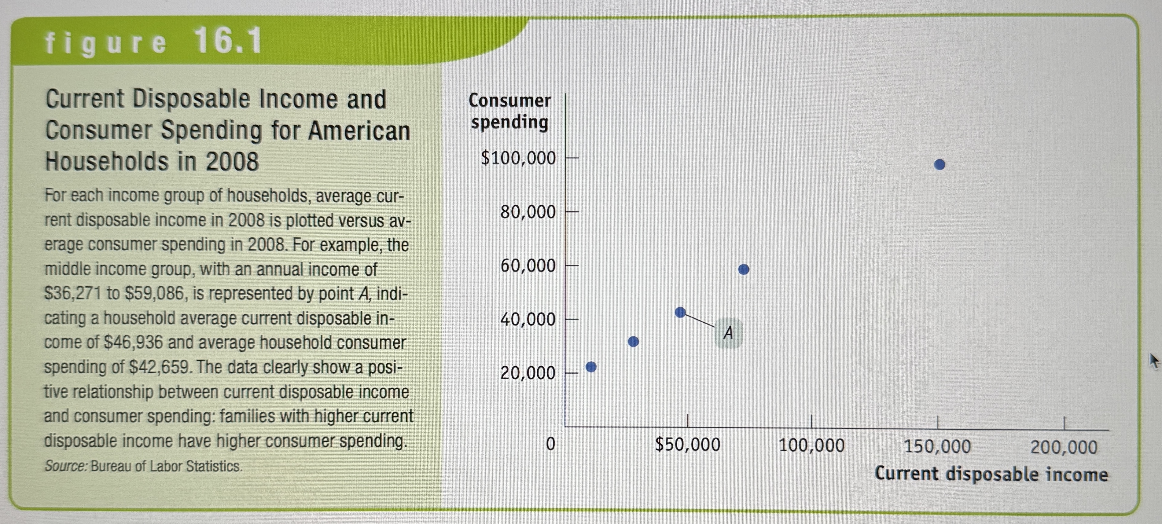
Current Disposable Income and Consumer Spending for Households (2008)
Ex.
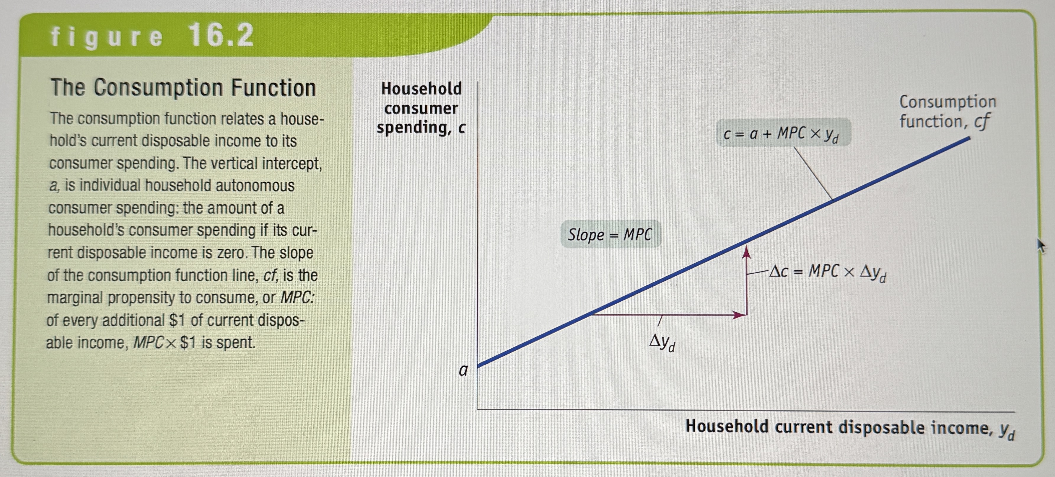
The Consumption Function
An equation showing how an individuals households consumer spending varies with the household‘s current disposable income.
Autonomous consumer spending
The a Constant. The amount of money a household would spend if it had no disposable income.
The Consumption Function Graph
Ex.
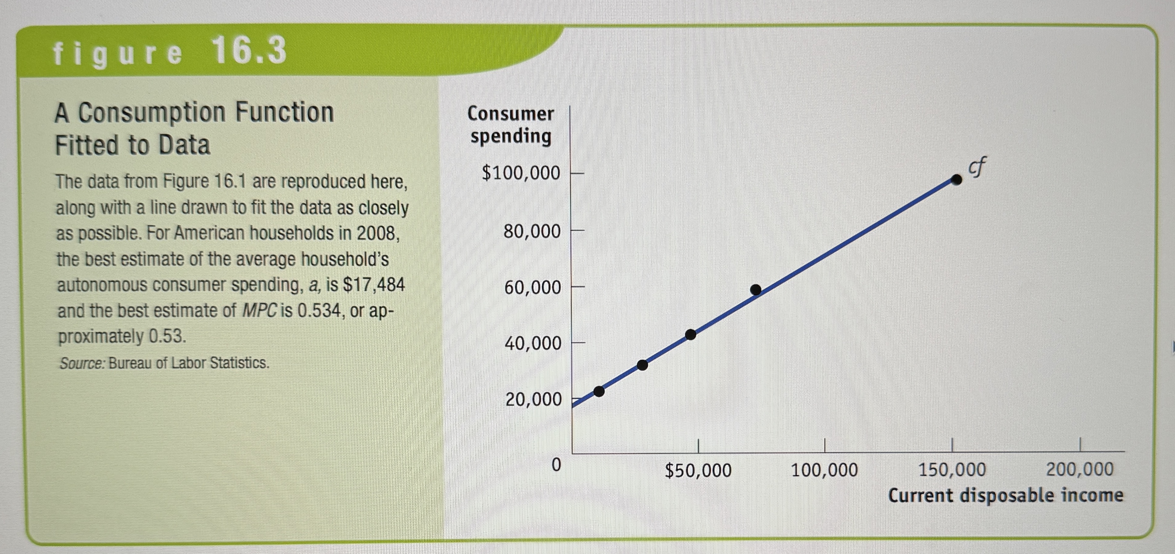
The Consumption Function Fitted to Data
Ex.
The aggregate consumption function
The relationship for the economy as a whole between aggregate current disposable income and aggregate consumer spending.
Shifts of the aggregate consumption function
Ex.
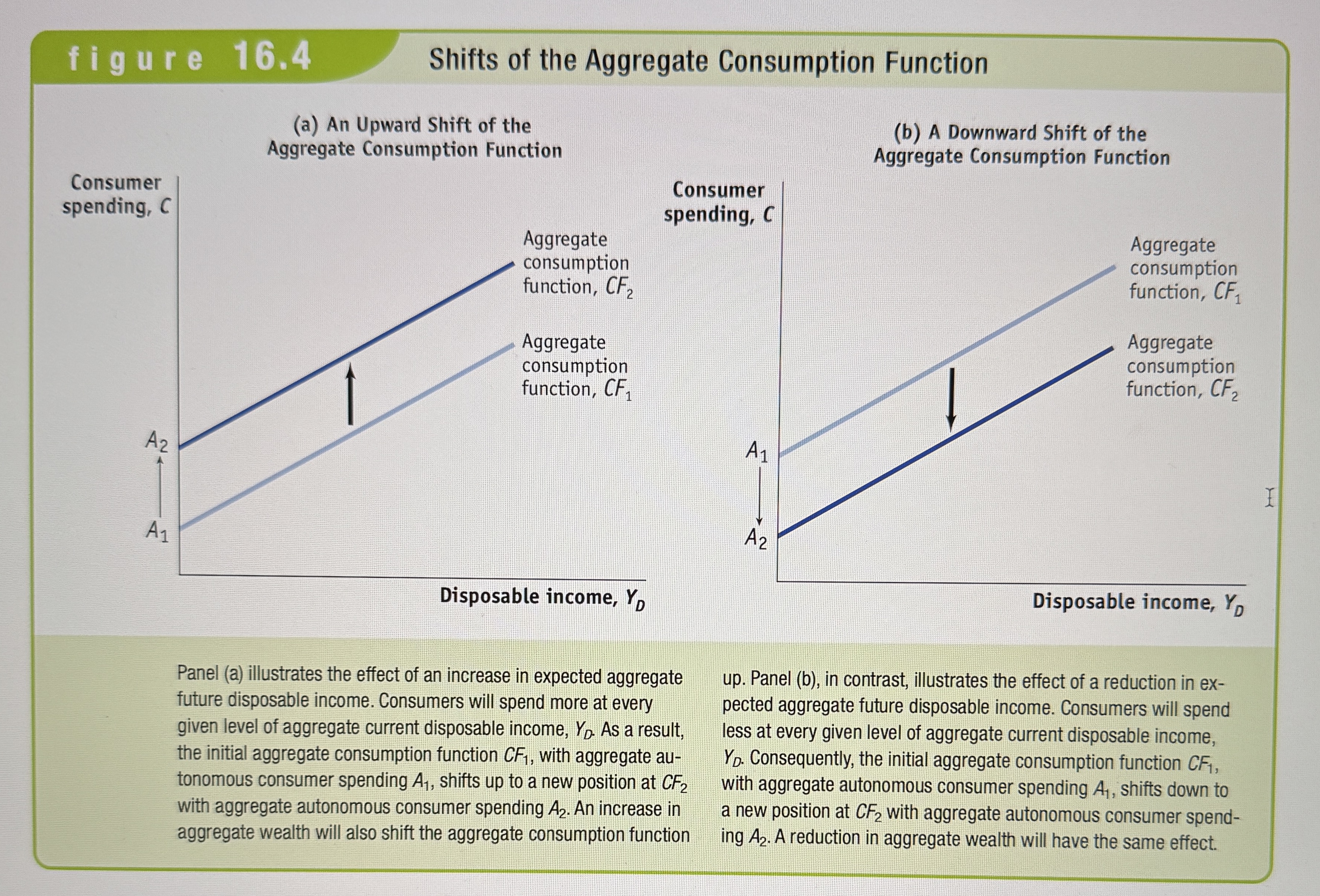
Shifts of the aggregate consumption function
Changes in expected future disposable income. If you expect your disposable income to rise in the future, then you are likely to not start spending on final goods and services right away.
Changes in aggregate wealth. People who have more wealth are more likely to spend more on consumption even if they have the same disposable income. Lifecycle hypothesis - consumers plan their spending over their lifetime not just in response to their current disposable income.
Planned Investment Spending
The investment spending that businesses intend to undertake during a given period.
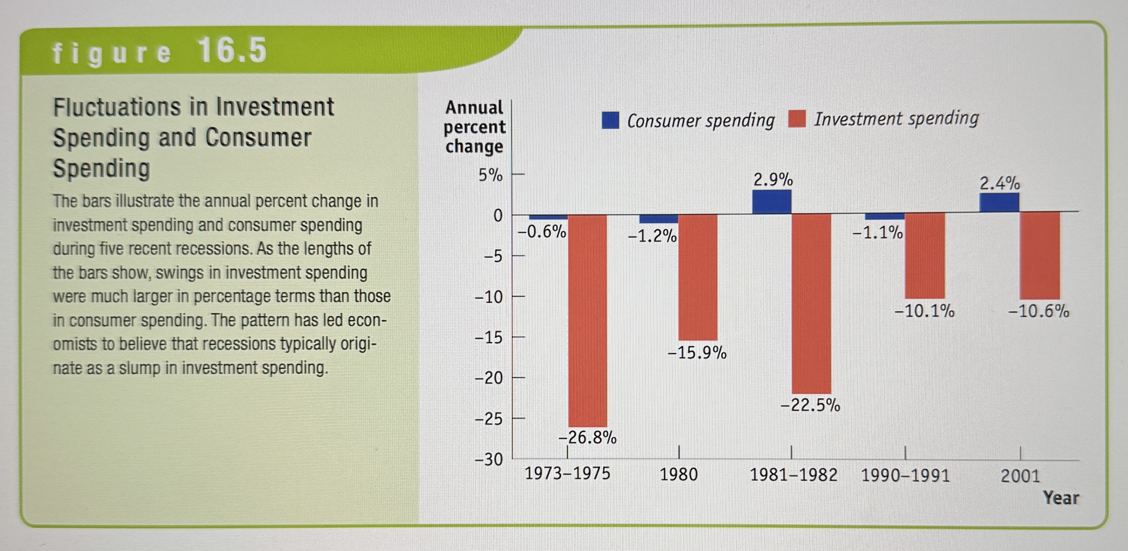
Fluctuations in investment spending and consumer spending
Ex.
Interest Rates and Construction
Interest rates have a direct impact on whether or not construction companies decide to invest in the construction of new homes.
Expected Real GDP, Production Capacity, and Investment Spending
A higher expected future growth rate of real GDP results in a higher level of planned investment spending, but a lower expected future growth rate of real GDP leads to lower planned investment spending.
Inventories
Stocks of goods held to satisfy future sales.
Inventory Investment
The value of the change in total inventories held in the economy during a given period.
Unplanned Inventory Investment
Positive unplanned inventory investment occurs when actual sales are less than businesses expected, leading to unplanned increases in inventories. Sales in excess of expectations result in negative unplanned inventory investment.
Actual investment spending
The sum of planned investment spending and unplanned inventory investment.
Interest Rate
An interest rate is the amount of money paid to a lender for borrowing money, or the amount paid to a saver for keeping money in a bank account.
The Aggregate Demand Curve
Shows the relationship between the aggregate price level, and the quantity of aggregate output demanded by households, businesses, the government, and the rest of the world.
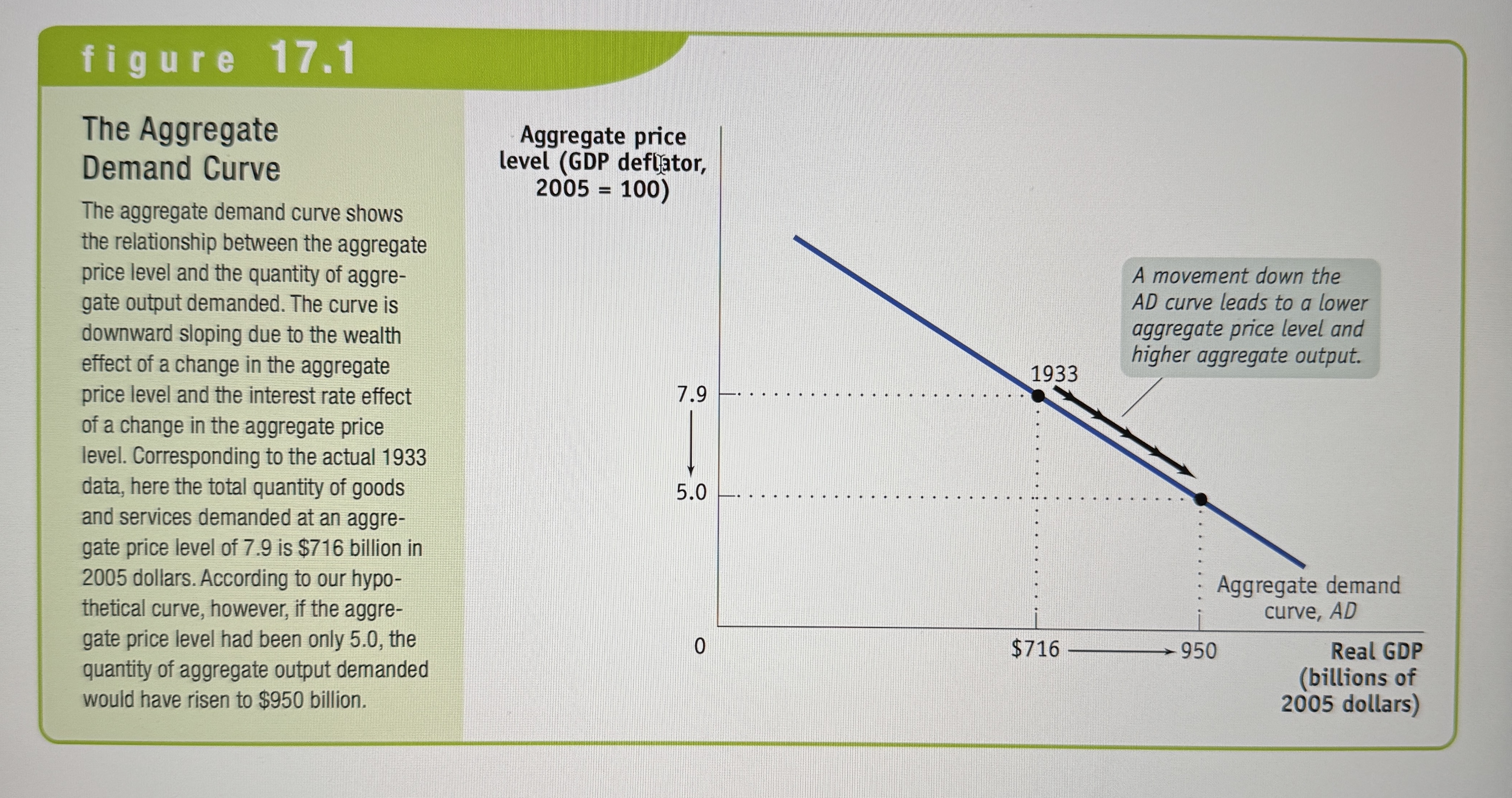
Why is the Aggregate Demand Curve Downward Slopping?
The aggregate demand curve is downward sloping because as the price level in an economy increases, consumers tend to buy less goods and services due to factors like the wealth effect, interest rate effect, and net export effect, leading to a decrease in overall aggregate demand at higher price levels.
The Wealth Effect
When prices rise, the purchasing power of people's money decreases, making them feel less wealthy and leading to reduced spending on goods and services.
The Interest Rate Effect
Higher price levels often lead to higher interest rates, which discourages borrowing and investment, further reducing aggregate demand.
Shifts on the Aggregate Demand Curve
Ex.
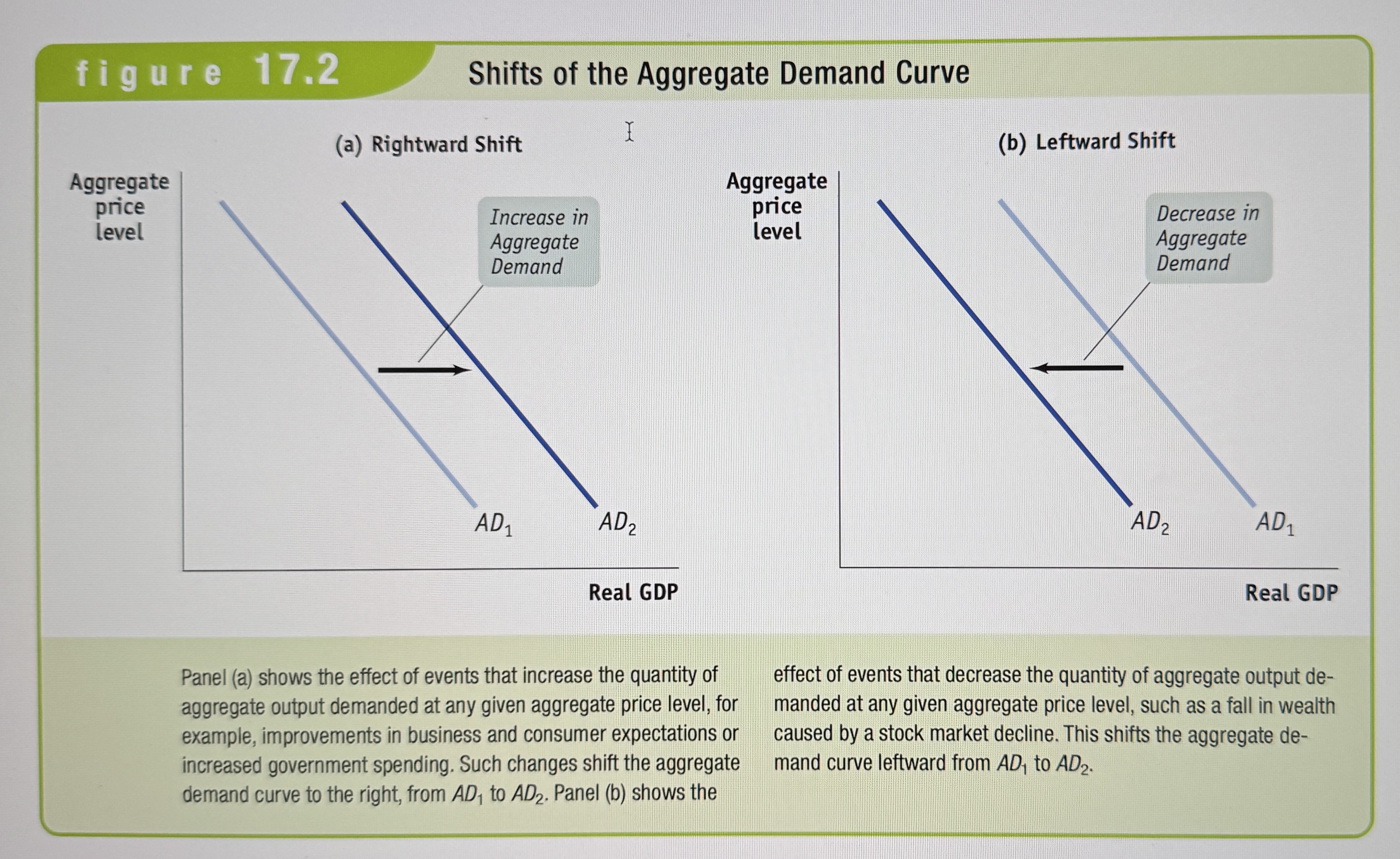
What are the shifters on the aggregate demand curve?
Ex.
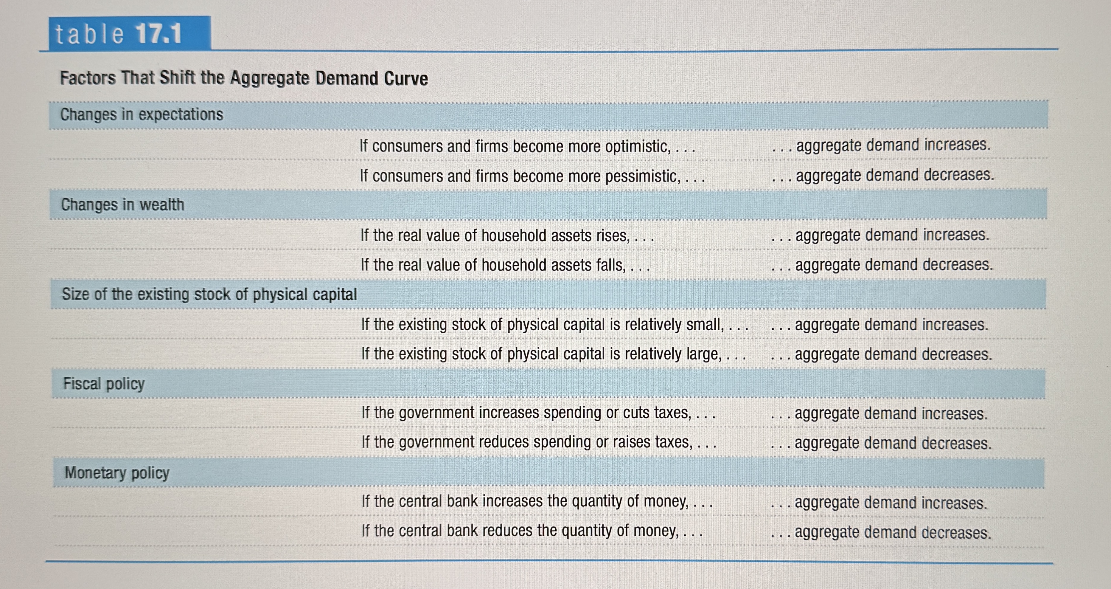
Fiscal Policy
The use of taxes, government transfers, or government purchases of goods and services to stabilize the economy.
Monetary Policy
The central banks use of changes in the quantity of money or the interest rate to stabilize the economy.
The Aggregate Supply Curve
Shows the relationship between the aggregate price level and the quantity of aggregate output supplied in the economy.
Why is there a short and long-run aggregate supply curve?
The key difference between the short-run aggregate supply (SRAS) curve and the long-run aggregate supply (LRAS) curve is that the SRAS is upward sloping, indicating that output can change with price level fluctuations in the short term due to factors like sticky wages, while the LRAS is a vertical line, showing that output remains fixed at full employment level regardless of price level changes in the long run when all factors can fully adjust.
Profit Per Unit
Price per unit of output - Production cost per unit of output
Nominal Wage
The dollar amount of the wage paid.
Sticky Wages
Nominal wages that are slow to fall, even in the face of high unemployment and slow to rise even in the face of labor shortages.
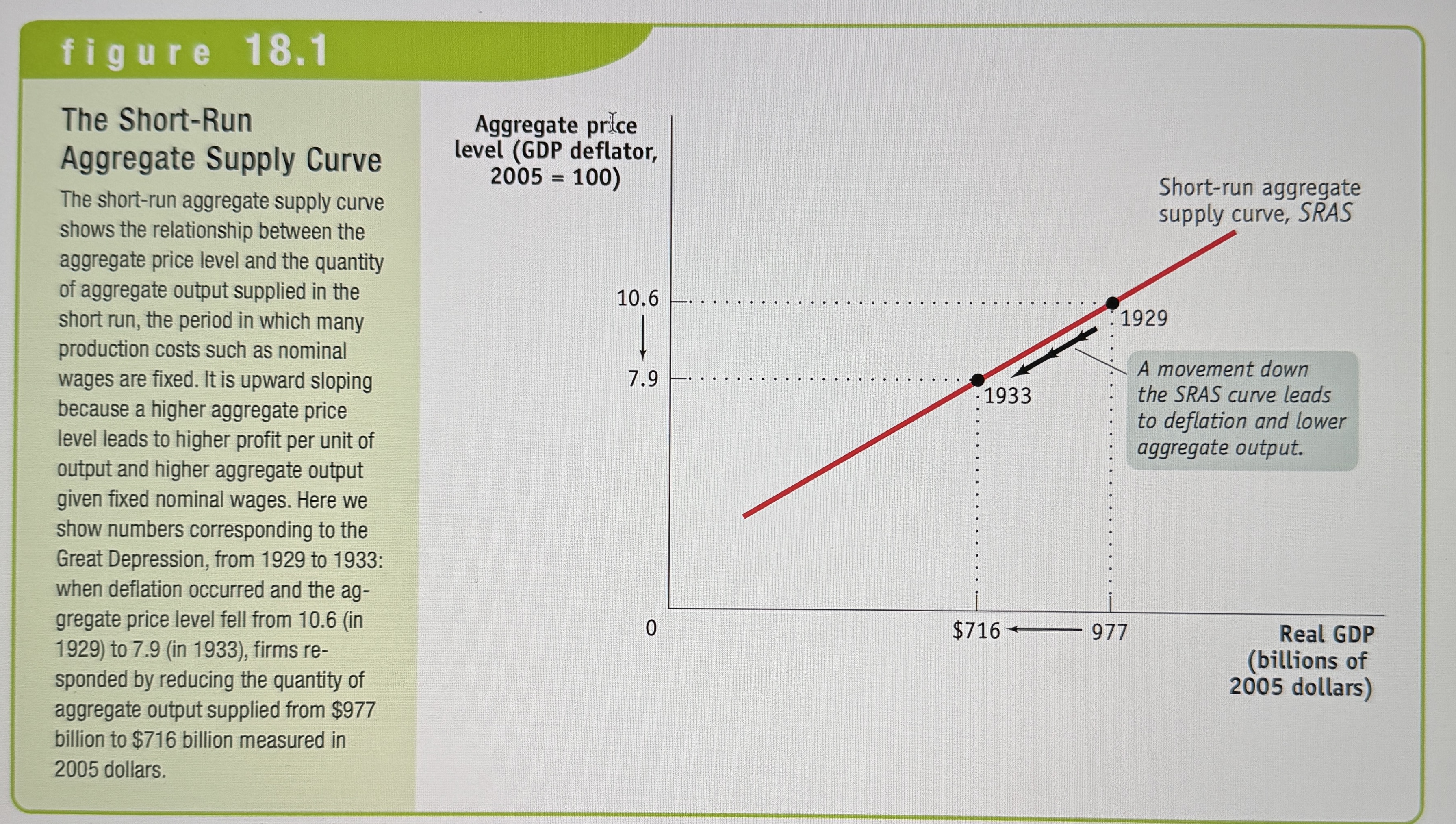
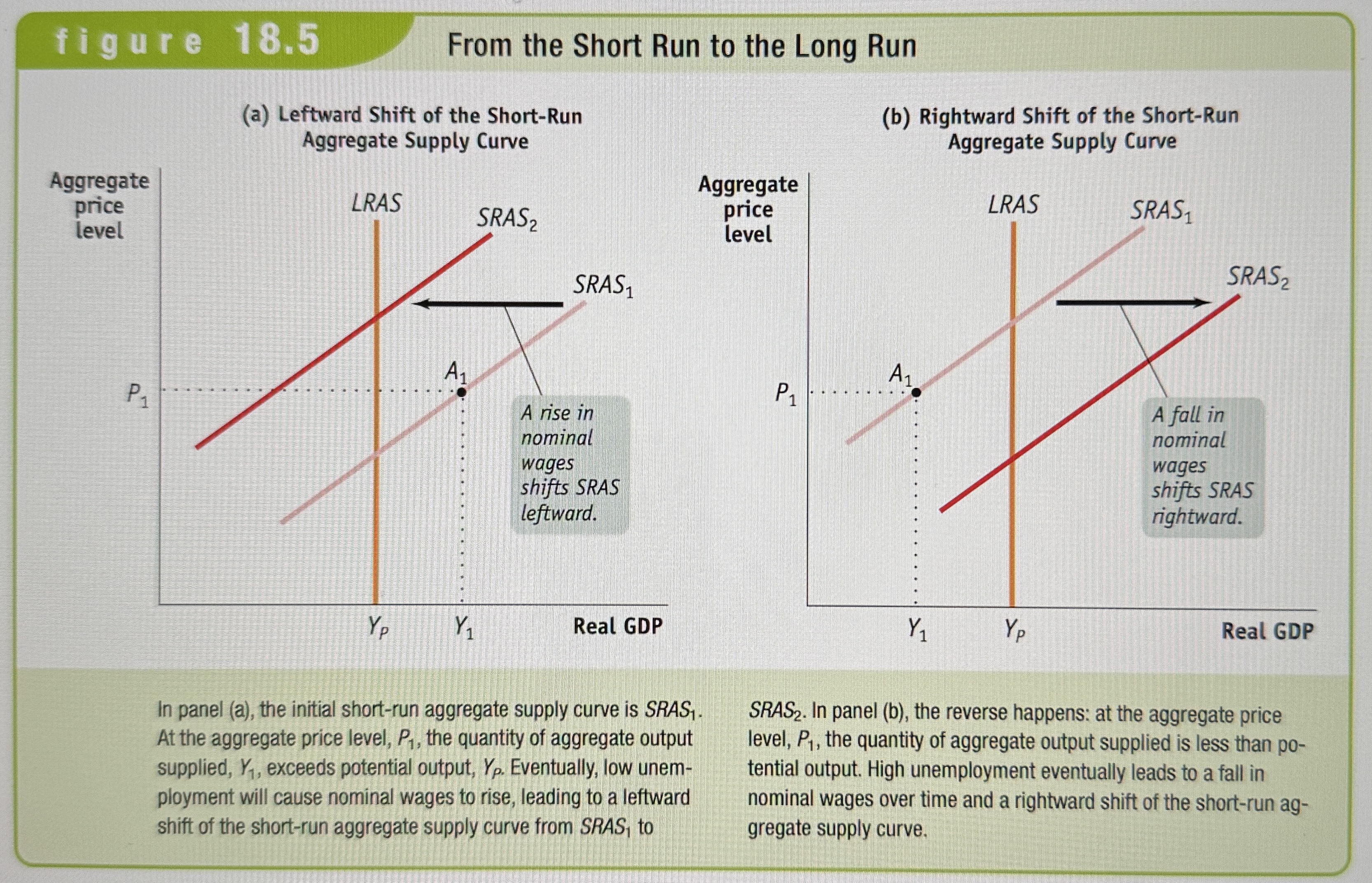
The Short-Run Aggregate Supply Curve
Shows the relationship between the aggregate price level and the quantity of aggregate output supplied that exist in the short run, the time period when many production costs can be taken as fixed.
Shifts on the Short-Run Aggregate Supply Curve
Ex.
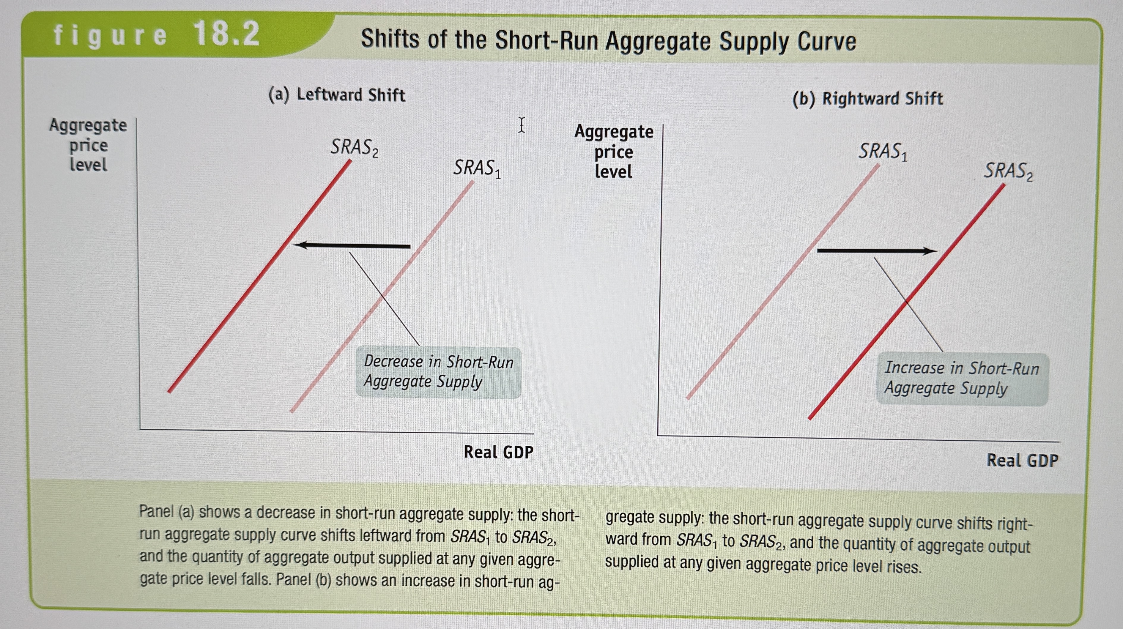
Factors that Shift the Short-Run Aggregate Supply Curve
The long-run aggregate supply curve
Shows the relationship between the aggregate price level and the quantity of aggregate output supplied that would exist if all prices, including nominal wages, we’re fully flexible.
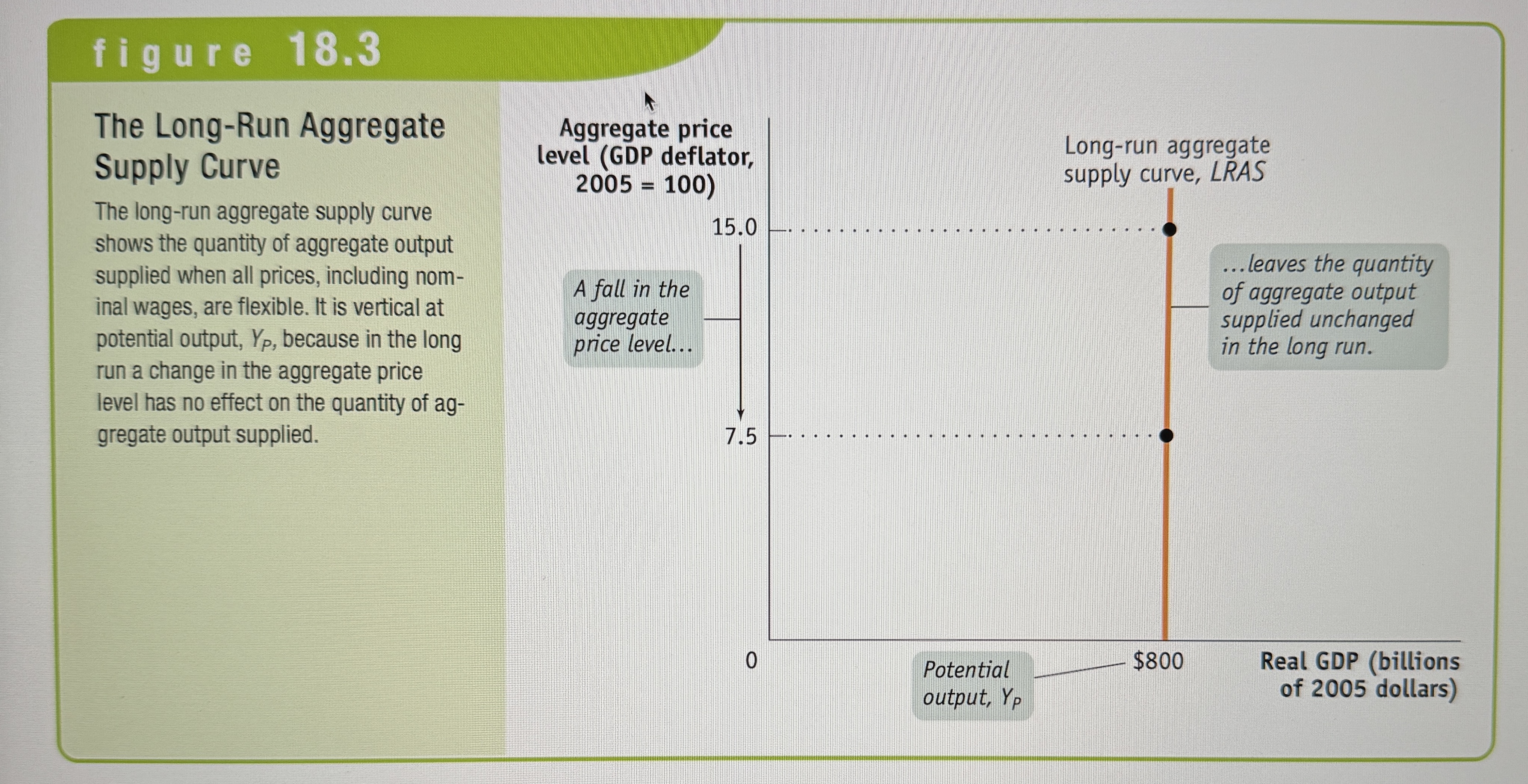
Potential Output
The level of real GDP the economy would produce if all prices, including nominal wages, were fully flexible.
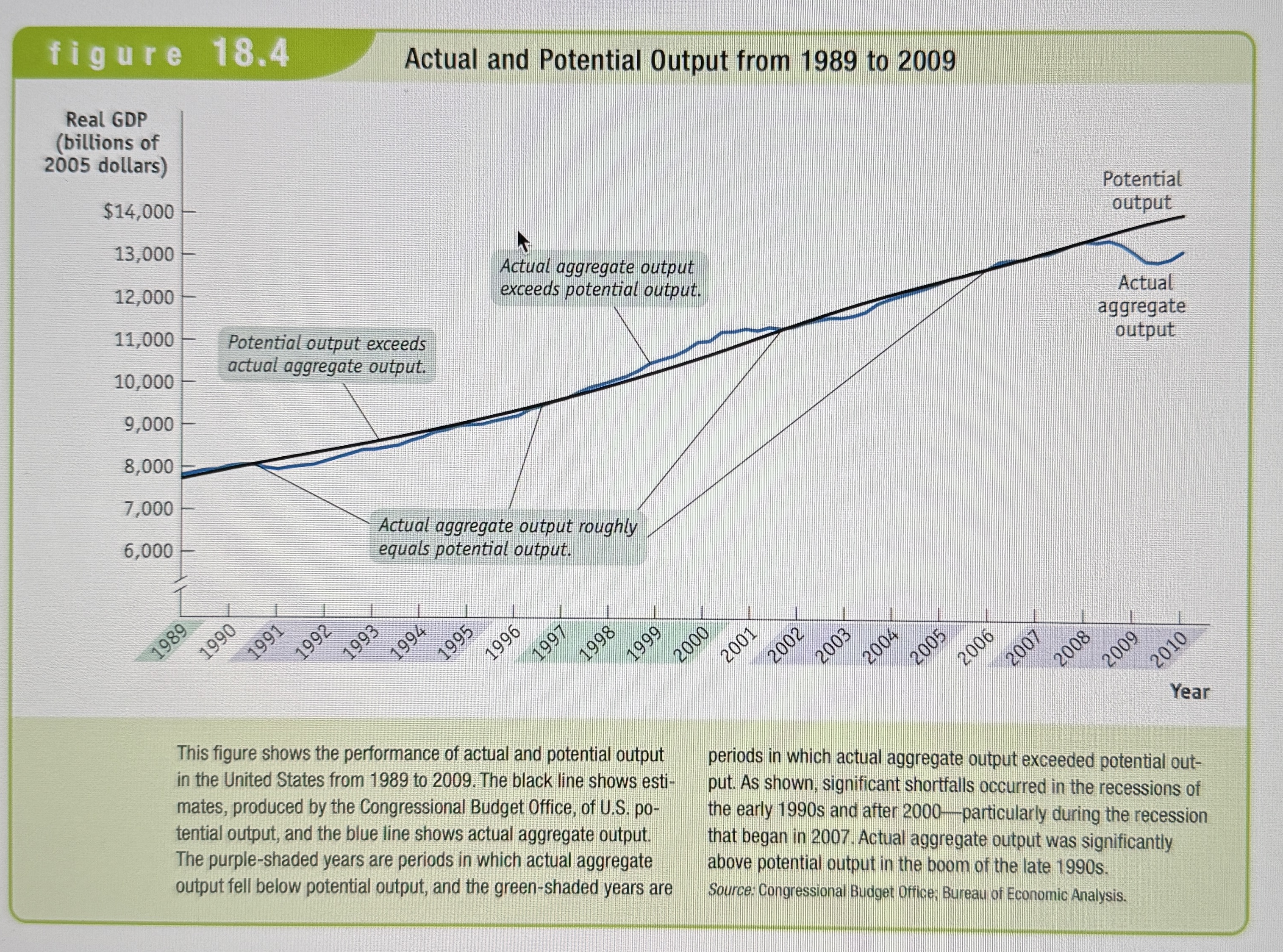
Actual vs Potential Output
Ex.
From Short Run to Long Run
Ex.
The AD-AS Model
In the AD-AS model, the aggregate supply curve and the aggregate demand curve are used together to analyze economic fluctuations.
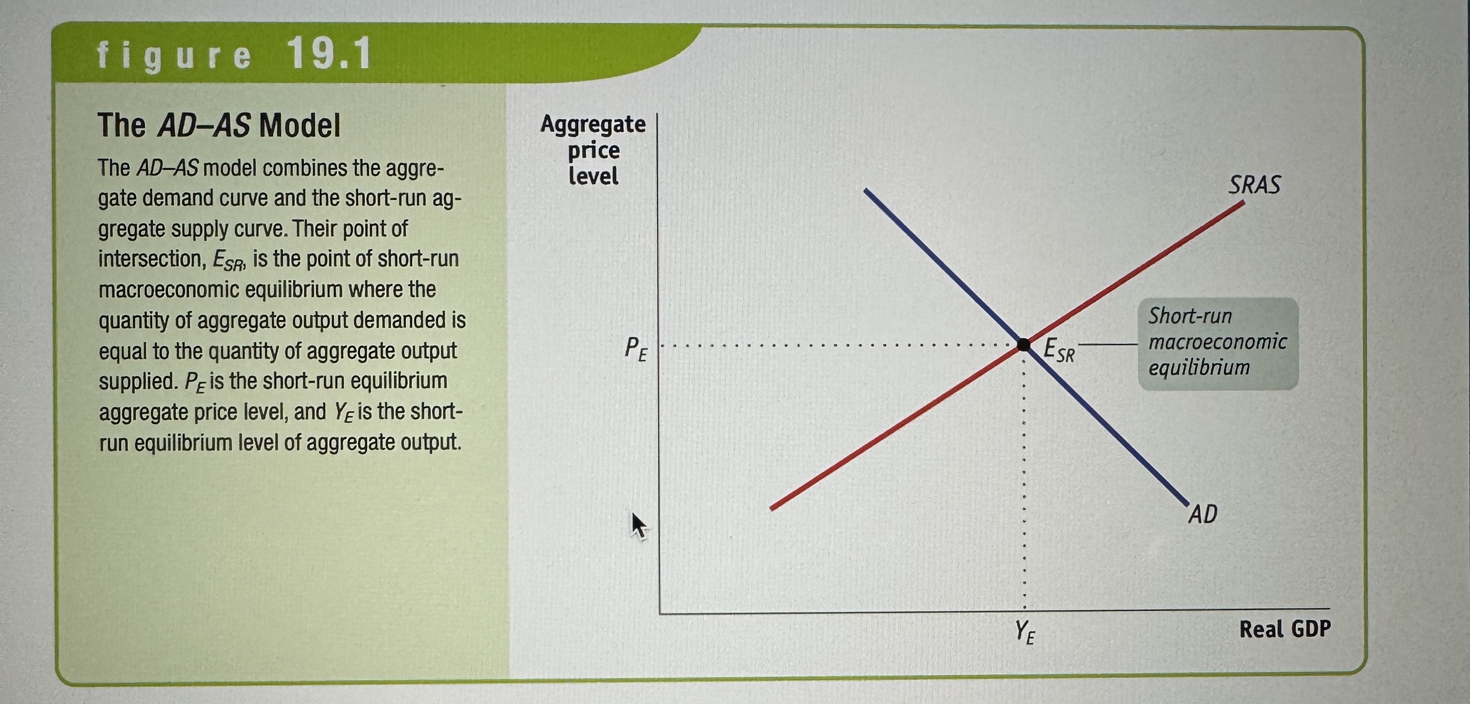
Short-Run Macroeconomic Equilibrium
The economy is in short-run macroeconomic equilibrium when the quantity of aggregate output supplied is equal to the quantity demanded.
Short-run equilibrium aggregate price level
The short-run equilibrium aggregate price level is the aggregate price level in the short-run macroeconomic equilibrium.
Short-run equilibrium aggregate output
The quantity of aggregate output produced in the short-run macroeconomic equilibrium.
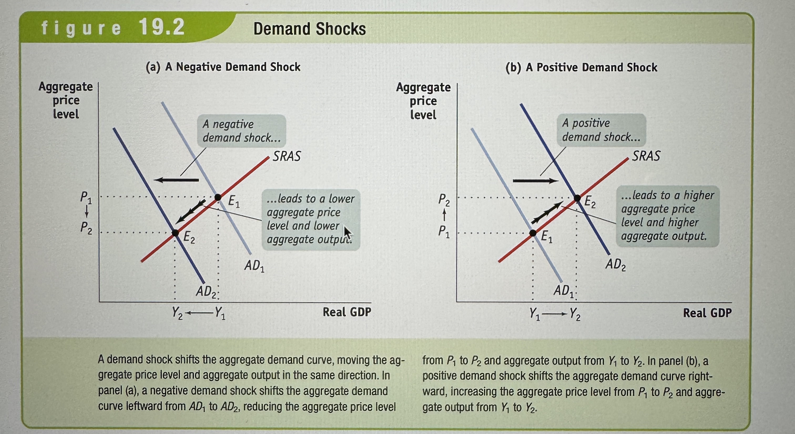
Demand Shock
An event that shifts the aggregate demand curve.
Supply Shock
An event that shifts the short-run aggregate supply curve.
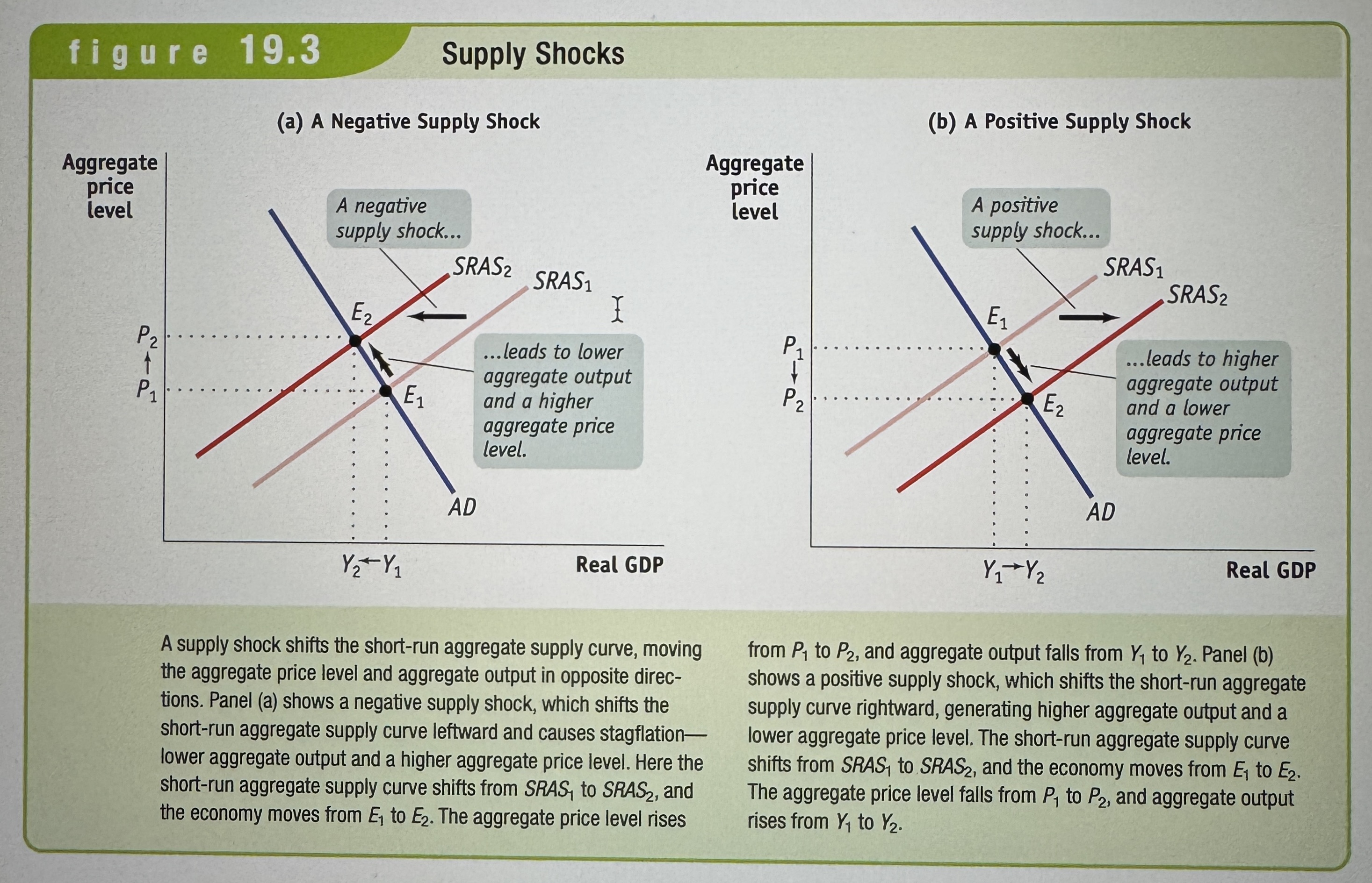
Stagflation
Stagflation is the combination of inflation and stagnating (or falling) aggregate output.
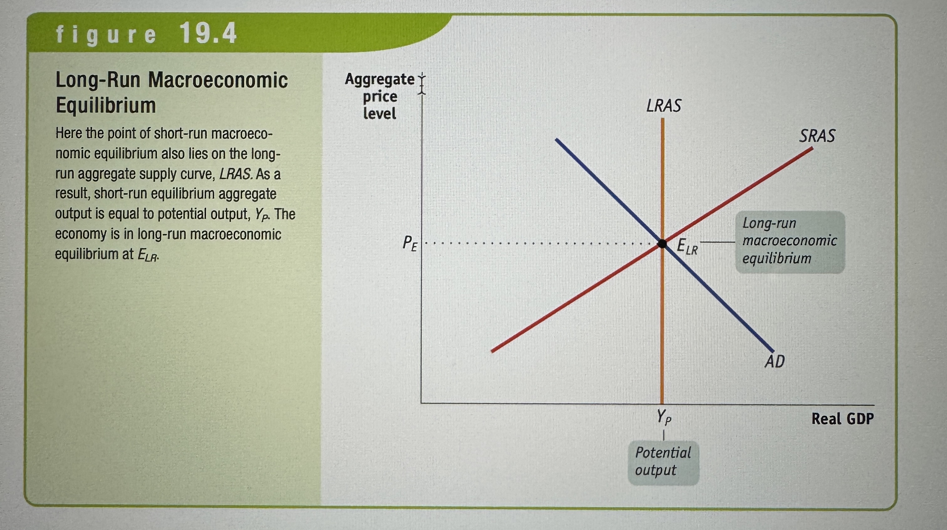
Long-run macroeconomic equilibrium
The economy is in long-run macroeconomic equilibrium when the point of short-run macroeconomic equilibrium is on the long-run aggregate supply curve.
Short-Run Versus Long-Run Effects of a Negative Demand Shock
Ex.
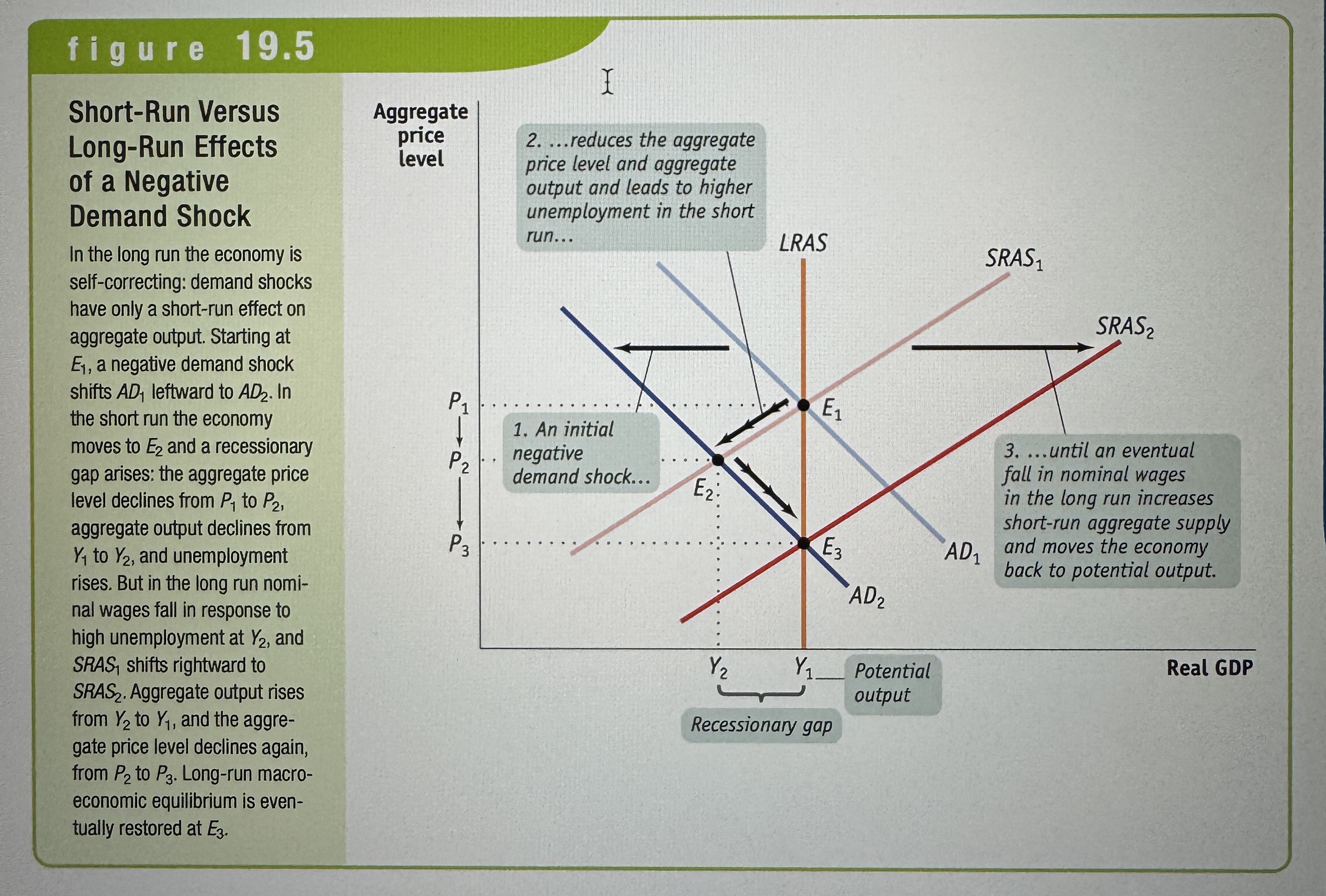
Recessionary Gap
There is a recessionary gap when aggregate output is below potential output.
Short-Run Versus Long-Run Effects of a Positive Demand Shock
Ex.
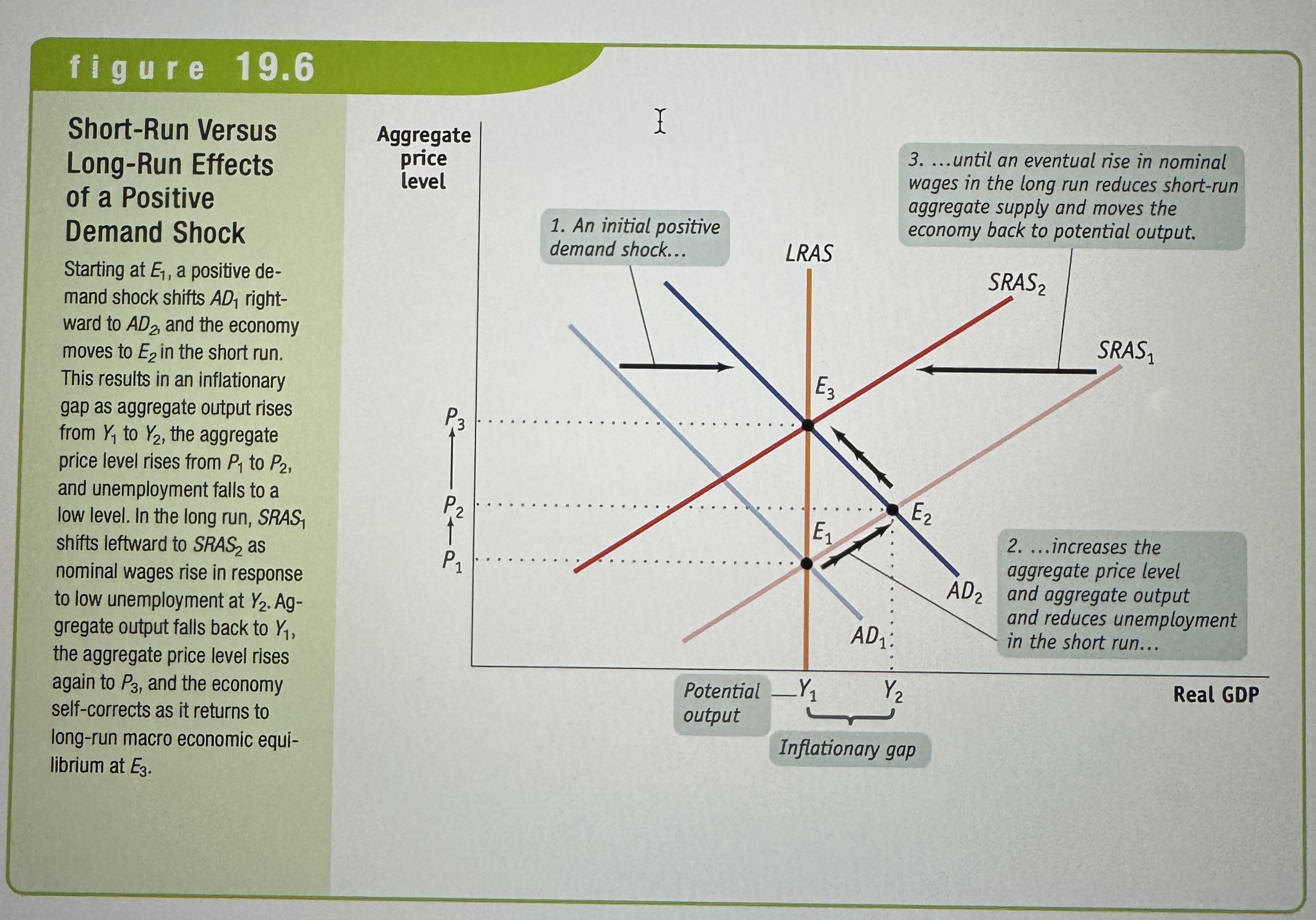
Inflationary Gap
There is an inflationary gap when aggregate output is above potential output.
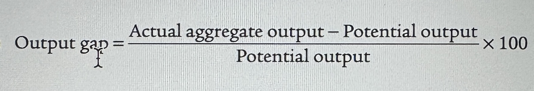
The Output Gap
The output gap is the percentage difference between actual aggregate output and potential output.
A self-correcting economy
The economy is self-correcting when shocks to aggregate demand affect aggregate output in the short run, but not the long run.
Stabilization Policy
The use of government policy to reduce the severity of recessions and rein in exclusively strong expansions.
Policy in the Face of Demand Shocks
Policy in the Face of Demand Shocks
Negative Demand Shock:
A leftward shift in the aggregate demand
(AD) curve reduces output and lowers prices.Quick monetary or fiscal action can shift
AD back right, restoring equilibrium.Benefits of Immediate Intervention:
Avoids Output Decline &
Unemployment: Prevents the temporary drop in output and associated rise in unemployment.Maintains Price Stability: Stops deflation, which is generally undesirable.
Considerations & Limitations:
Long-Run Costs: Some measures (e.g., increased budget deficits) may harm long-run growth.
Policy Uncertainty: Imperfect information and unpredictable effects mean that interventions could sometimes create more instability.
Positive Demand Shocks: Even though higher output and lower unemployment seem beneficial, short-run gains from an inflationary gap can lead to long-run costs; thus, both negative and positive shocks are typically countered.
Policy Preference:
Modern practice favors monetary policy over fiscal policy for smoothing out both recessionary and inflationary gaps.
Policy in the Face of Supply Shocks
Responding to Supply Shocks
Effects of a Negative Supply Shock:
Decreases aggregate output (higher unemployment).
Increases aggregate prices (inflation).
Policy Challenges:
Unlike demand shocks, no government policy can easily reverse shifts in production costs.
Using monetary or fiscal policy to shift aggregate demand creates a trade-off:
Increasing AD can lessen
unemployment but worsens inflation.Decreasing AD can curb inflation but increases unemployment.
Real-World Choices:
Policymakers in the 1970s (and similarly in early 2008) often prioritized price stability over low unemployment, accepting higher unemployment as a trade-off.
Fiscal Policy Basics
Fiscal policy is the way by which the government can manipulate the nation's economy. They do this in two ways:
Through government spending
Through taxation
There are two types of fiscal policy and they include expansionary fiscal policy and contractionary fiscal policy. Expansionary fiscal policy refers to laws that increase output by either increasing government spending or decreasing taxes. Contractionary fiscal policy refers to laws that decrease inflation by decreasing government spending or increasing taxes.
Social Insurance
Programs made by the government intended to protect families against economic hardship.
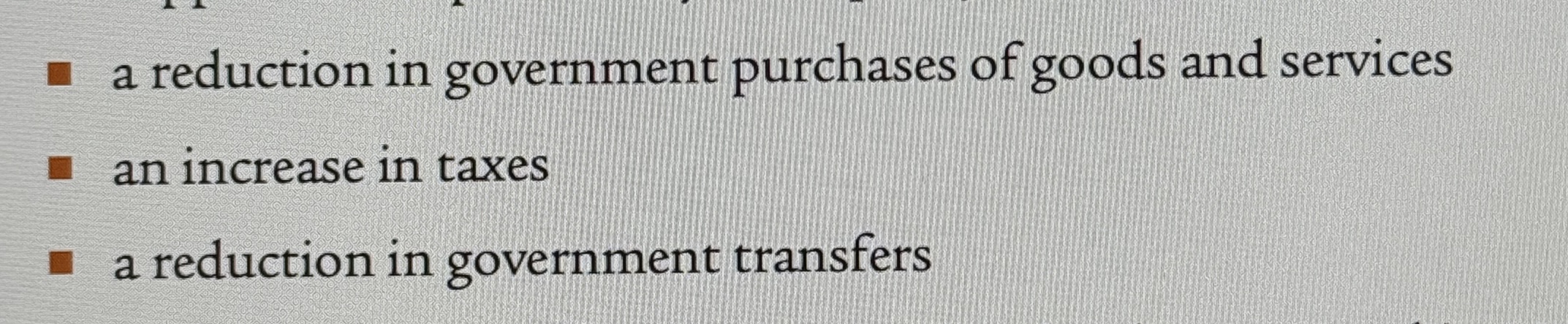
Expansionary Fiscal Policy
Expansionary Fiscal Policy
Ex.

Contractionary Fiscal Policy
Ex.
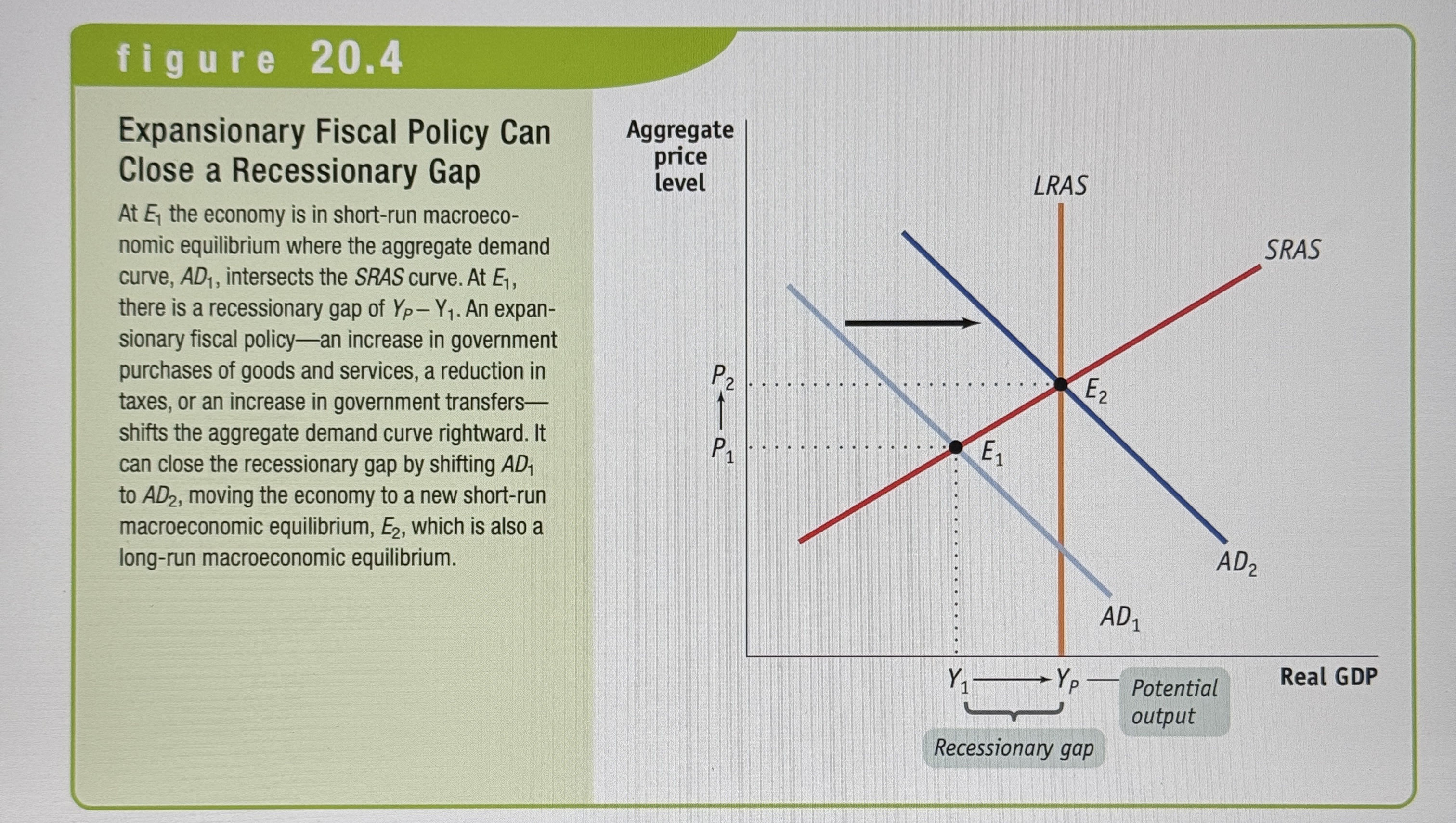
Expansionary Fiscal Policy Can Close a Recessionary Gap
Ex.
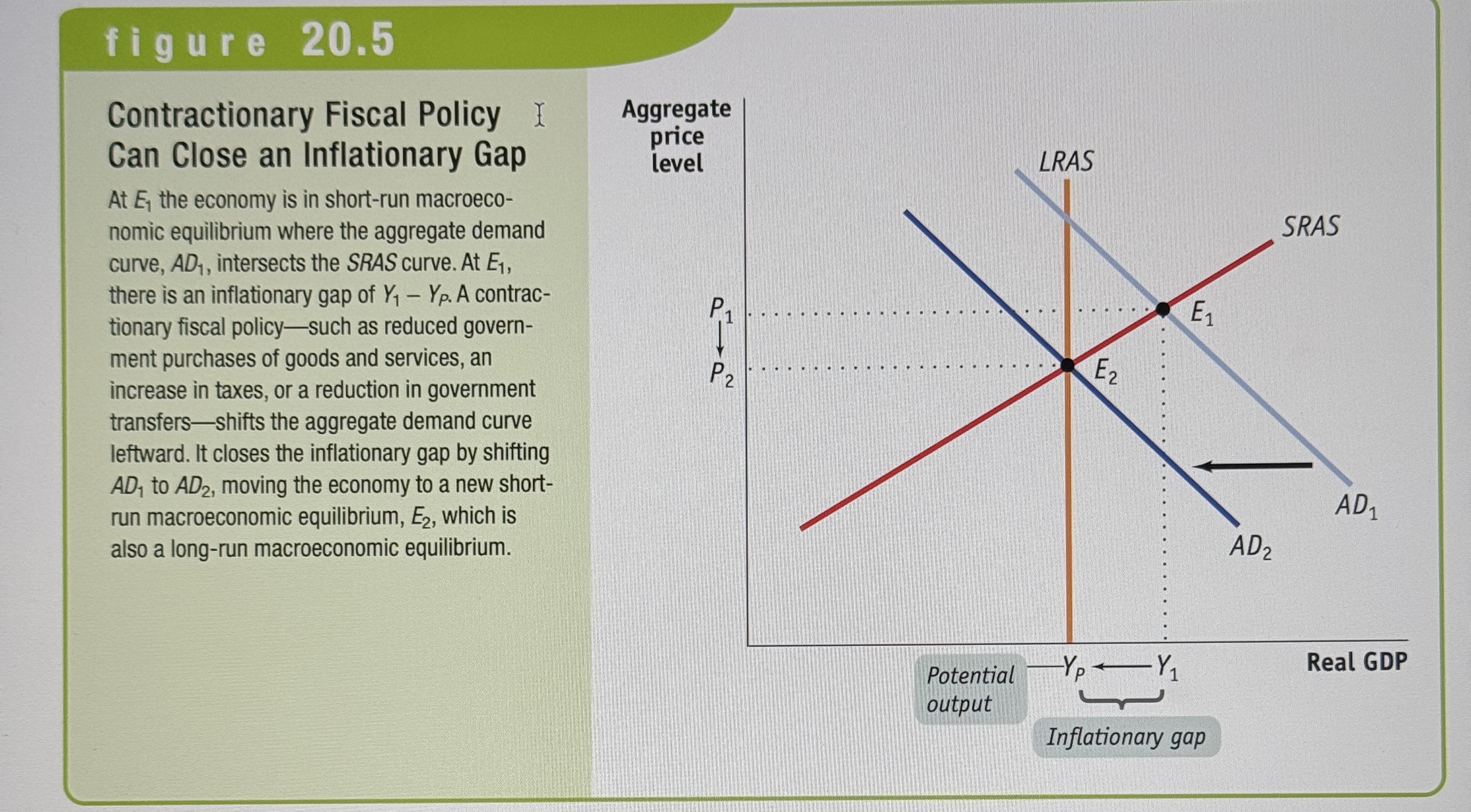
Contractionary Fiscal Policy Can Close an Inflationary Gap
Ex.
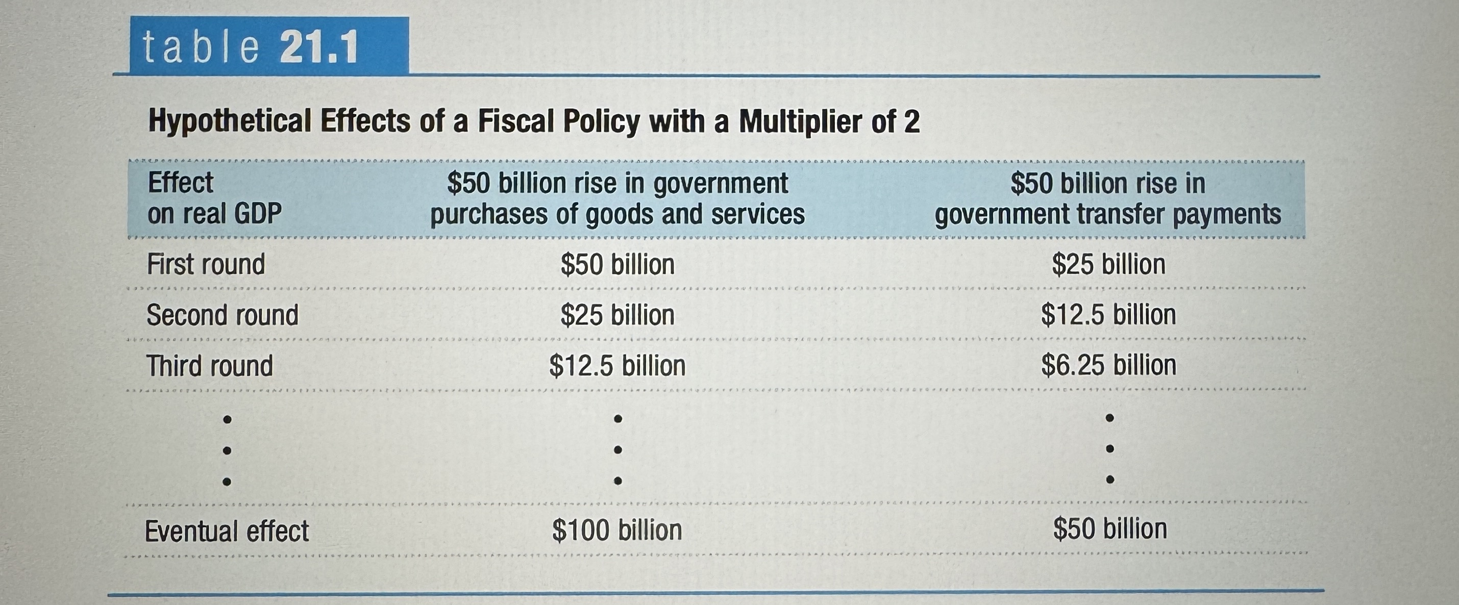
Fiscal Policy and Multipliers
If we said that the MPC was .5, then that means that the MPS is also .5. If you remember MPC + MPS always equals 1. The spending multiplier is calculated by dividing 1/MPS. So in this particular situation, the spending multiplier would be 2. This means that for every dollar the government spends, it will multiply twice in the economy.
Lump-sum Taxes
Taxes that don’t depend on the taxpayers income.
Automatic Stabilizera
Government spending and taxation rules that cause fiscal policy to be automatically expansionary when the economy contracts and automatically contractionary when the economy expands.
Discretionary fiscal policy
Fiscal policy, that is the result of deliberate actions by policymakers rather than rules. For example, during a recession, the government may pass legislation that cuts taxes and increases government spending in order to stimulate the economy.
More on fiscal policy and multipliers…
Fiscal policy has a multiplier effect on the economy, the size of which depends upon the fiscal policy. Except in the case of lump-sum taxes, taxes reduce the size of the multiplier. Expansionary fiscal policy leads to an increase in real GDP, while contractionary fiscal policy leads to a reduction in real GDP. Because part of any change in taxes or transfers is absorbed by savings in the first round of spending, changes in government purchases of goods and services have a more powerful effect on the economy than equal-size changes in taxes or transfers.