FDA PP Answers

T/F - . Fourier series can never be used to smooth non-periodic data.

FALSE; they can be used as they can accommodate variations from periodicity

T/F - The degrees-of-freedom of a penalised smoother is always less than the number of basis functions used to smooth the data.

TRUE; as penalisation creates more constraints

T/F - When performing function on function regression if one uses a concurrent model the slope parameter is a scalar.

FALSE; it is a function

T/F - The mean squared error is always smaller than variance.

FALSE; MSE also includes bias so equal to or greater than var

T/F - If we are using a harmonic acceleration roughness penalty, the resulting x(t) becomes exactly periodic as λ → 0.

FALSE; It becomes exactly periodic when λ → ∞

T/F - For a B-spline one can increase the number of basis functions, either by increasing the number of knots or by increasing the order of spline.

TRUE; nbasis = number of internal knots + order

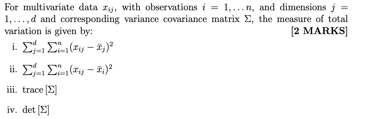
i and iii

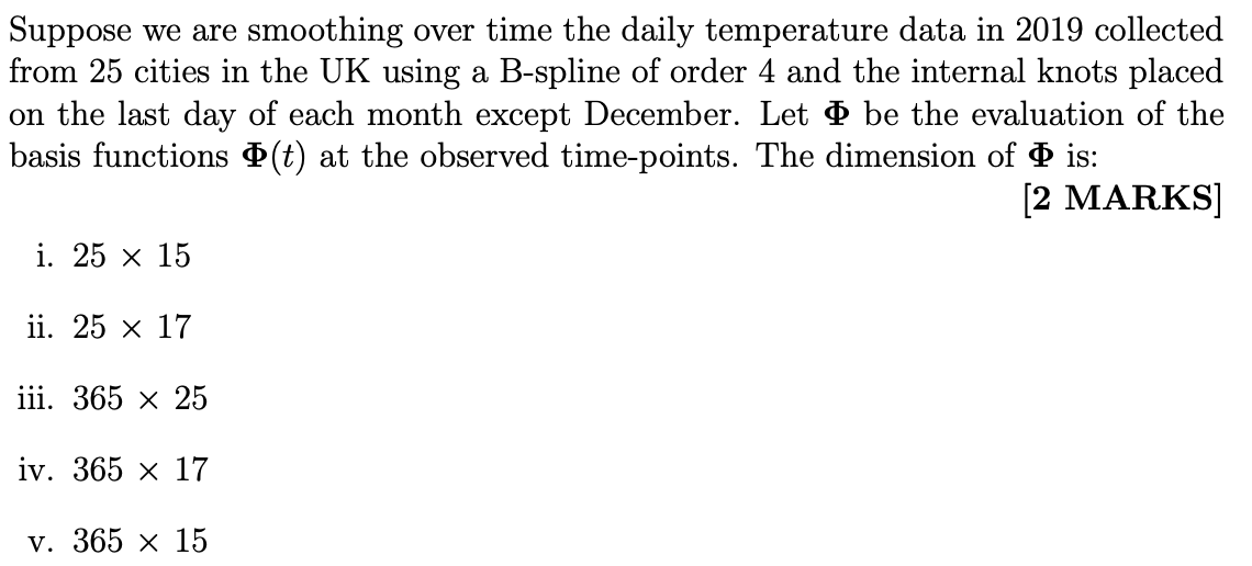
(v); rows = number of time points , columns (number of basis function = internal knots (11)+ order (4) = 15

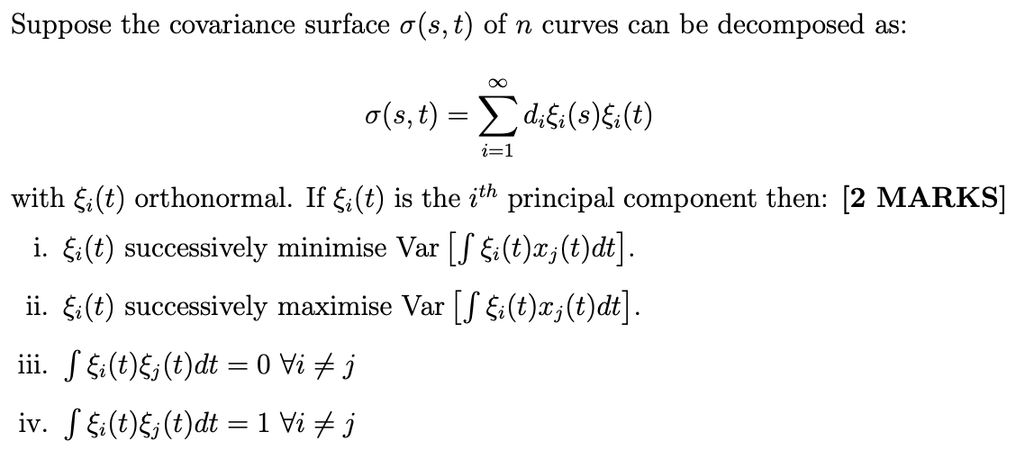
i and iii

Let tempfd be a functional data object obtained by using the smooth.basis function in the fda package.

The code plot(deriv.fd(tempfd$fd))

will plot the

first derivative of the curve

Suppose you have observed data at 81 equally spaced time points on a single curve. The dataset is given by y0, y1, y2, . . . , y80 corresponding to time-points t = 0, . . . , 80 (a) If you are using a saturated Fourier basis, how many basis functions do you need to use?

(b) Write the expressions for the first 3 and the last 2 basis functions in the saturated Fourier basis.

© Write the R code using functions from fda to create the saturated Fourier series

(d) Can you obtain a continuous fourth derivative of the fitted curve if you just used 3 Fourier basis to fit the curve? Justify your answer.

(a) 81

(b) 1, sin(ωt), cos(ωt) sin(40ωt), cos(40ωt)

© timerange=c(0,80) create.fourier.basis(timerange,81)

(d) Yes, Smoothing with Fourier series have infinite derivatives

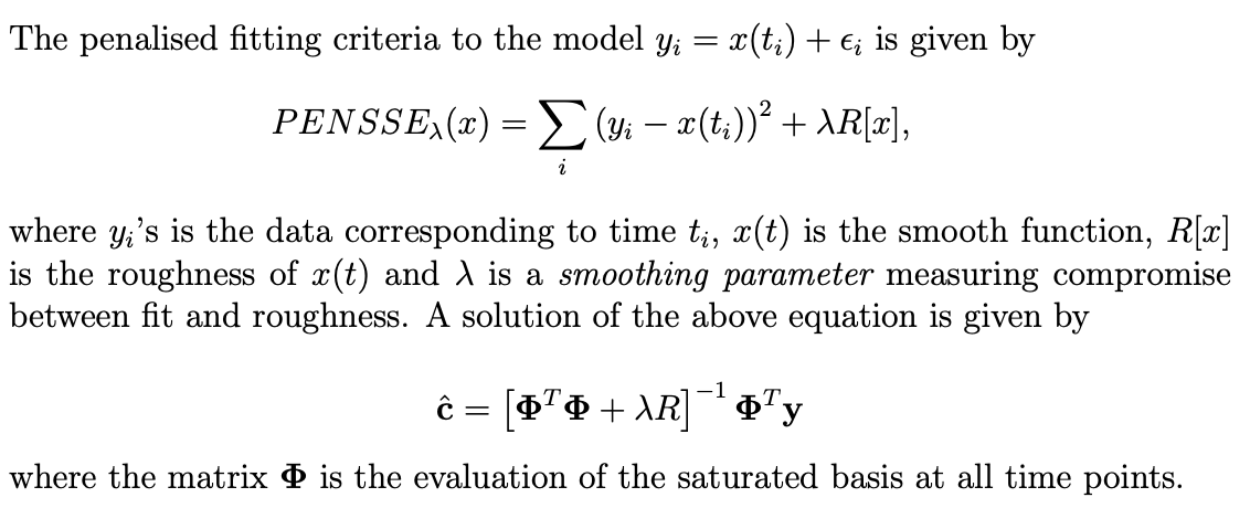
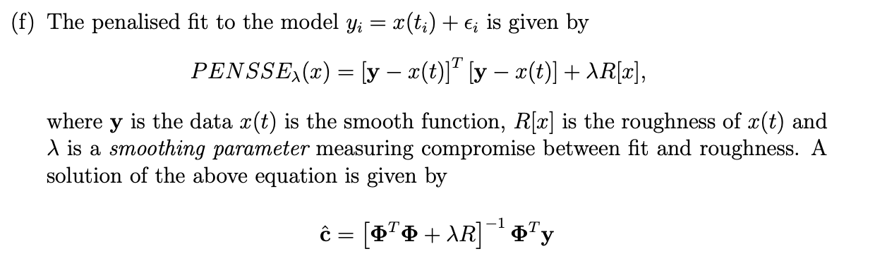
i. What are the dimensions of c, Φ, R and λ?

ii. Write the expression of R in terms of the basis function Φ(t) for a harmonic acceleration penalty. Hint: You do not need to workout the actual derivatives

iii. Name the functions in the fda library that you need to use to fit the penalised smoother to the data.

iv. Let yˆ be the fitted value of y using the penalised fit with harmonic acceleration penalty. Express yˆ in terms of y, Φ, R and λ and argue that yˆ is a linear smoother.

(i) c → 81 × 1, Φ → 81 × 81, R → 81 × 81 and λ → 1 × 1

Describe, the steps specifying the relevant functions from the fda library that you would need to test the null hypothesis, that the rate of change in growth in the two types of chicken is the same.

• Smooth the data by Choosing an appropriate basis function. One should use a b-spline basis or a basis with monotone increase as we are modelling growth curve. create.bspline.basis()

• Use smooth.basis to smooth the data either by using a penalised or unpenalised estimator

• Take the derivative of the growth curve using the function derv.fd for the two groups

• Two perform the hypothesis test of whether the two rates of growths are same one cane use the function tperm.fd to perform a two sample t-test for functional objects among the two groups are same vs they are different

• Alternatively, one can use the regression setting with the group as a indicator variable and test the hypothesis of β(t) = 0 using the function Fperm.fd

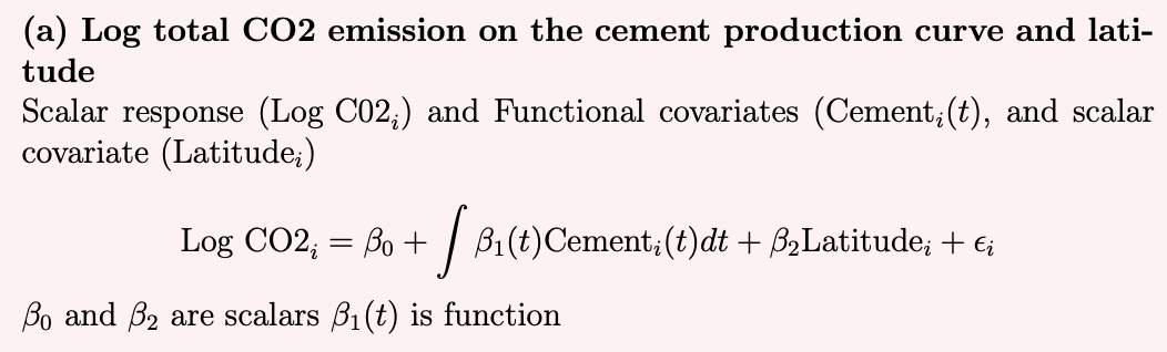
(a) Log total CO2 emission on the cement production curve and latitude.

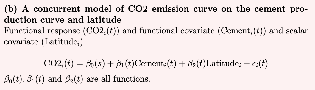
(b) A concurrent model of CO2 emission curve on the cement production curve and latitude.

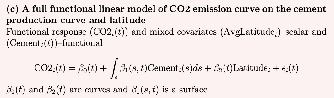
(c) A full functional linear model of CO2 emission curve on the cement production curve and latitude.

T/F - A cubic spline basis with no internal knots is the same as a polynomial basis

TRUE; they can be used as they can accommodate variations from periodicitysimilar to third order polynomial fit

T/F - The degrees-of-freedom of a penalised smoother increases with increase in the magnitude of penalty paramater .

FALSE; degrees-of-freedom of a penalised smoother decreases

T/F - When performing function on function regression if one uses a historical model the slope parameter is a surface.

TRUE; Surface

T/F - Fitting smooth curves is just linear regression using basis functions as independent variables

TRUE

T/F - The bases of fourier series of any order is orthogonal to each other

TRUE

Suppose we are smoothing the temperature data observed every 5 days in 2010 of 50 cities in the UK using a B-spline of order 3 and knots placed every time point. Let Φ be the evaluation of the basis functions Φ(t) at the observed time-points. The dimension of Φ is:

365 X 15 ; rows = number of time points 365/5=73, columns (number of basis function = internal knots (72)+ order (3) = 75

Let waterfd be a functional data object obtained by using the smooth.basis function in the fda package.

The code plot(deriv.fd(waterfd$fd,2)) will plot the:

i. smooth curve

ii. smooth curve with linetype 2

iii. first derivative of the curve

iv. second derivative of the curve

iv

Suppose you have observed data at 11 equally spaced time points on a single curve.

The dataset is given by y0, y1, y2, . . . , y11 corresponding to time-points t = 0, . . . , 10

(a) If you are using a cubic b-spline with internal knots at t = 3, 6, 8 how many basis function do you have.

(b) Using this example or in general prove that you cannot fit a unpenalized cubic spline if you put a knot at every time-point.

(c) What is the maximum number of adjacent intervals each of the basis functions of a cubic spline can have positive support on

(d) The R code from fda library to create b-spline takes the following argument (rangeval=___, nbasis=___, norder=___, breaks=___) Write the code for defining a cubic spline basis with knots at every time point using

(i) Only the arguments (rangeval=___, nbasis=___, norder=___)

(ii) Only the arguments (rangeval=___, nbasis=___, breaks=___)

(iii) Only the arguments (rangeval=___, norder=___, breaks=___)

(e) What order of spline should you use if you wish to calculate the third order derivative of the curve

(a) 4 + 3 = 7

(b) resulting number of basis 9+4=13, but only 11 data points

© 4 same as order

(d) > a1=create.bspline.basis(rangeval = c(0,10),nbasis=13,norder = 4)

> a2=create.bspline.basis(rangeval = c(0,10),nbasis=13, breaks = 0:10)

> a3=create.bspline.basis(rangeval = c(0,10),norder=4, breaks = 0:10)

(e) order 5

i. Write the expression of R for a fourth derivative penalty

ii. What are the dimensions of c, Φ, R and λ?
iii. Name the functions in the fda library that you need to use to fit the penalised smoother to the data.

iv. State at least two approaches of determining an optimal value of λ

Suppose we have data on the daily covid cases (over 6 months) with similar testing capacity from 30 countries, 10 from each of the 3 continents Asia, Europe and South America. We wish to find out if there is difference in how the disease has progressed in the three continents. Accounting for the difference of population and the first case of the diseases we should ideally look at the rate of change

Describe, the steps specifying the relevant functions from the fda library that you would need to test the null hypothesis, that the rate of change covid cases in the three continents are similar.

• Smooth the data by Choosing an appropriate basis function. One can use any basis e.g. create.bspline.basis()

• Use smooth.basis to smooth the data either by using a penalised or unpenalised smoother

• Take the derivative of the growth curve using the function deriv.fd for each of the 30 countries

• Use the regression setting with the group as a indicator variable and test the hypothesis of µ1(t) = µ2(t) = µ2(3) using the function Fperm.fd

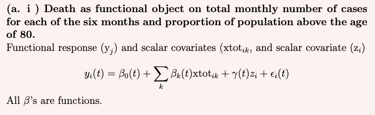
i. Death as functional object on total monthly number of cases for each of the six months and proportion of population above the age of 80.

ii. A concurrent model of Death as functional object on the smoothing the daily number of cases and proportion of population above the age of 80.

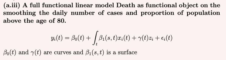
iii. A full functional linear model Death as functional object on the smoothing the daily number of cases and proportion of population above the age of 80.

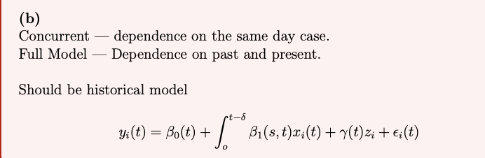
(b) Given the fact that Deaths follow cases, and there is a lag between the number of cases and the number of deaths, do you think the concurrent model in part (ii) or the full functional model in (iii) is appropriate. Justify your answer and propose an alternative model and write it out as a functional linear model. [

T/F - An order 4 B-spline basis with exactly one internal knot is the same as a cubic polynomial basis.

FALSE; It would be true if there was not an internal knot

T/F - The degrees-of-freedom of a penalised smoother with the penalty parameter λ = 0 is exactly same as the number of basis functions.

TRUE; If penalty parameter is non-zero dof < number of basis

T/F - When performing a functional regression of a single response function on another functional explanatory variable, if one uses a concurrent model the slope parameter is a surface.

FALSE; function

T/F - For a Fourier basis one can increase the number of basis functions, either by increasing the number of knots or by increasing the order of spline.

FALSE; true for B-splines

T/F - Functional principal components are always orthogonal to each other

FALSE; Not orthogonal for penalised versions

T/F - For any linear smoother both OCV (ordinary cross validation) and GCV (generalised cross validation) have a closed form expression.

TRUE

(b) Suppose we are temporally smoothing the weekly total covid cases, for 52 weeks in 2021 for 20 cities in the UK using a B-spline of order 5 and knots placed every week.

Let Φ be the evaluation of the basis functions Φ(t) at the observed timepoints of a particular city. The dimension of Φ is …. × ….

(c) The B-spline basis in functions in part(b) will be positive over at most … adjacent intervals.

(d) As the knots belonging to the B-spline in part (b) are distinct, it will have continuous derivative up to degree ...

(b) rows = number of time points 52; columns (number of basis function = internal knots (51)+ order (5) = 56

© 5

(d) 3

(e) Let covidfd be a functional data object obtained by using the smooth.basis function in the fda package.

The code plot(deriv.fd(covidfd$fd,3)) will plot the …

Third derivative of covidfd

(f) The function … in the fda package will allow us to evaluate the value of the functional object covidfd at 10 distinct time points.

evalfd

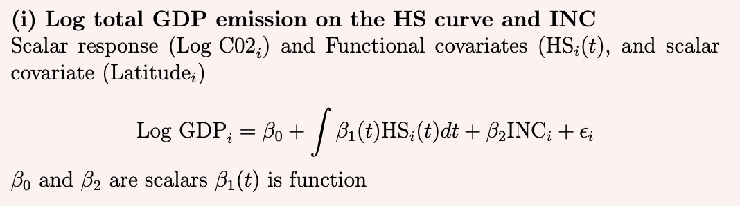
i. Log total GDP on HS curve and Income

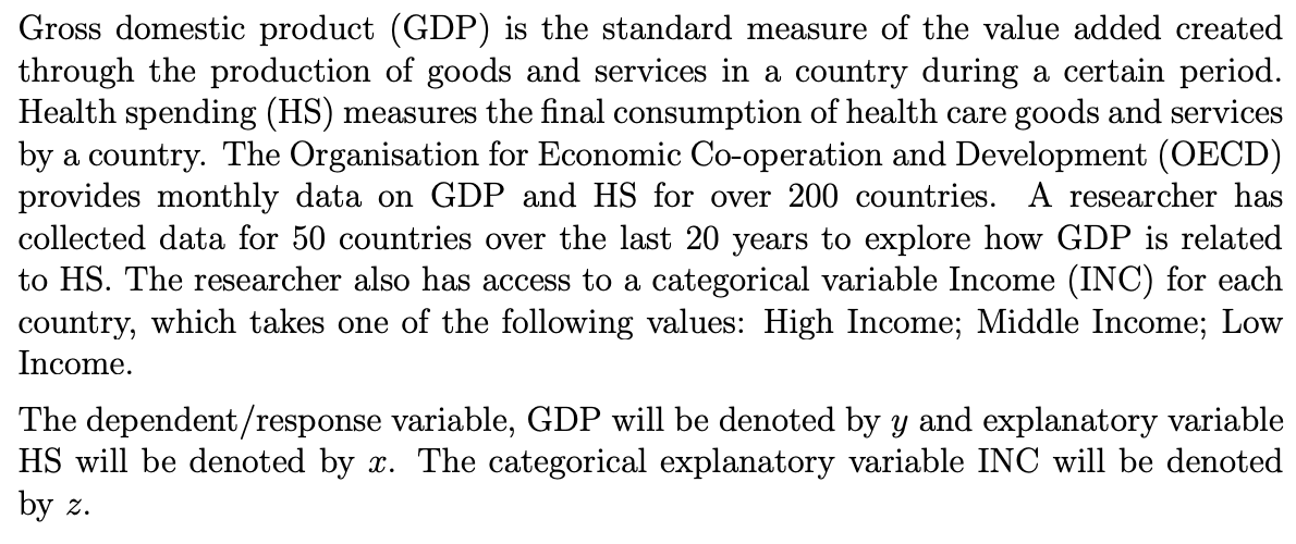
ii. A concurrent model of GDP curve on HS curve adjusting for the level of INC of the country.

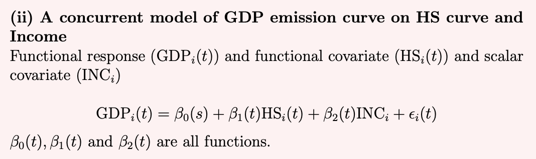
iii. A full functional linear model of GDP curve on the HS curve adjusting for the level of INC of the country.

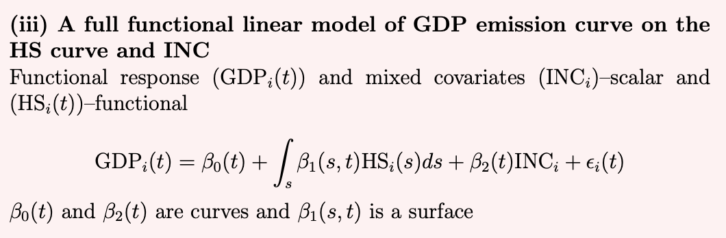
iv. A functional linear model of GDP curve on the yearly HS totals adjusting for the level of INC of the country.

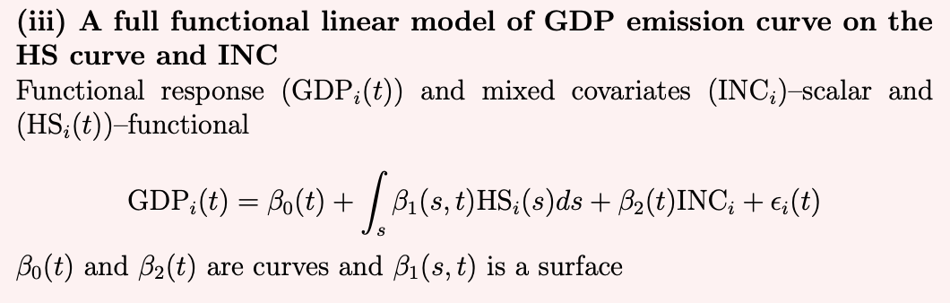
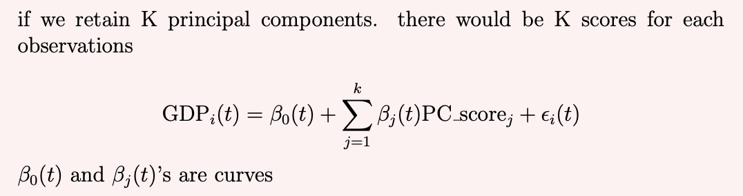
Instead of using the HS curve, if you choose to use the first 4 functional Principal Components score of the HS curve as explanatory variables and the GDP curve as the response variable, how will your analysis differ from part a (iii) in terms of the model and dimensions of β’s.

Make a list of the R functions and describe the steps you will need to implement part (b) using the fda package.

create.fourier.basis or create.bspline.basis smooth.basis pca.fd fRegress

• Smooth both curves using

• Perform a pca on the HS curves

• Look at the scree plot/variation explained and retain k components

• Calculate the score functions

• Perform a function on scalar/multivariate regression on each of the principal components

why a classical two-sample t-test is not appropriate for comparing growth curves (i.e. functional data, not scalar data)

• Classical t-tests require scalar/vector inputs.

• Applying them pointwise causes correlation and multiple testing issues.

• Distributional assumptions on entire curves are hard to verify.

• There is an infinite hypothesis testing problem when working with functions.

Why are the pointwise critical values different for each time point?

Even though n1n​ and n2n stay the same across time:

• The variability in the data (sample variances) at each time point changes.

• This causes the approximate degrees of freedom to change.

• Hence, the critical values of the t-test differ pointwise.

Hypothesis Test for Mean Growth Curves

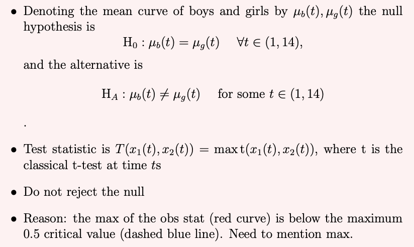
How would you modify the code tperm.fd(hgtmfd,hgtffd) to test the hypothesis that the rate of growth of boys and girls are the same? [2

tperm.fd(deriv.fd(hgtmfd,1),deriv.fd(hgtffd,1))

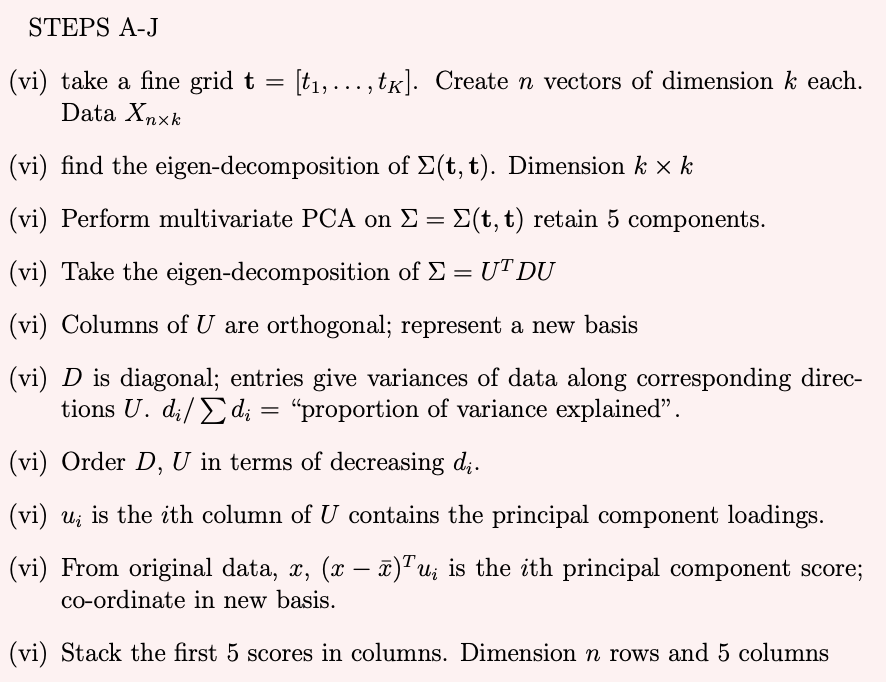
Suppose you are restricted from using functional principal component techniques. Show the steps for obtaining the projection of the curves X1(t), . . . , Xn(t) on the first 5 principal component directions using techniques from multivariate principal components. At each step specify the dimension of the matrices.

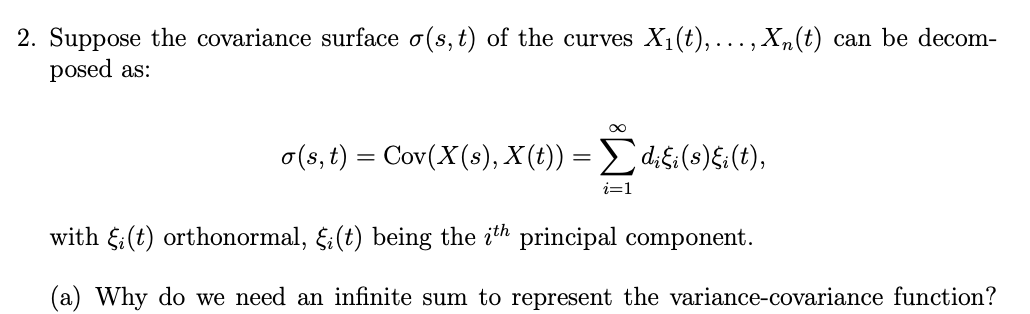
In general σ(s, t) Represents continuous surface in two dimensions so we need infinite sum to represent all possible variance covariance functions.

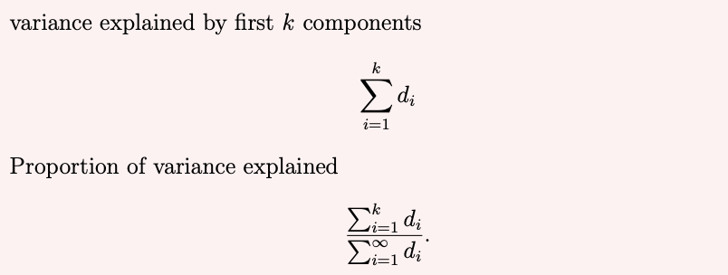
Derive an expression for the proportion of variance explained by the first k principal components.

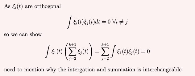
Show that the first functional principal component is orthogonal to the sum of k following principal components.

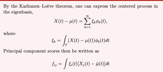
(d) Denoting µ(t) as the mean of X1(t), . . . , Xn(t), find an expression for the principal component score of the j th observation on the i th principal component. [5 M

What will be the dimensions of the principal components score matrix for the data on the first 5 functional principal components?

n rows and 5 columns

Functional data analysis can be applied to study not only temporal data but also spatial data, making it a versatile approach for understanding patterns varying over a continuum.

TRUE; The same techniques work support needs to be changed to space etc

. The degrees-of-freedom of a penalised smoother is less than or equal to the number of basis functions used to smooth the data.

TRUE; as penalisation creates more constraints the degrees of freedom is smaller or same

When performing functional regression the response variable can be a scalar, vector or function.

TRUE; FDA regression have different techniques for each of these situations

When regressing a scalar random variable on a functional covariate, we always need to penalize the fitted slope function.

TRUE; Otherwise it will not be identifiable

If we are using a harmonic acceleration roughness penalty, the resulting x(t) becomes exactly periodic as penalty paramater λ = 1.

FALSE; λ → ∞ the x(t) has no contribution from the data and defined entirely by the penalty function which is periodic

i. Keeping k and λ fixed, if the order is increased to p + 1 then the degrees of freedom changes to d + 1.

ii. Keeping p and λ fixed, if the number of knots is decreased to k − 2 then the degrees of freedom will be less than or equal to d.

iii. Keeping p and k fixed, if the penalty parameter λ is increased then the degrees of freedom will be greater than or equal to d.

iv. Fixing λ = 1, if the order is increased to p + 1 and the number of knots is decreased to k − 1 the degrees of freedom remains unchanged.

i) FALSE as it is penalized the increase might be less than 1 in degrees of freedom

ii) TRUE - degrees freedom will decrease with decrease in knots

iii) FALSE - degrees freedom d will decrease with increase in penalty

iv) FALSE - nbasis = number of internal knots + order and nbasis=degree of freedom for un-penalised estimators i.e. only for λ = 0