Spending and Output in the Short Run

The Keynesian Model

• Building block for current theories of short-run economic fluctuations and stabilization policies

• In the short run, firms meet demand at preset prices

  • Firms typically set a price and meet the demand at that price in the short run

    • Menu costs are the costs of changing prices

      • Determining the new price

      • Incorporating prices into the business

      • Informing consumers of new prices

• Firms change prices when the marginal benefits exceed the marginal costs

Technology of Changing Prices

• Technology has reduced menu costs 

  • Bar codes and scanners reduce costs of changing prices in the store

  • Online surveys

• Highly segmented airline pricing

• Internet mechanisms for setting price

  • eBay

  • Priceline

• Ride-sharing apps

• Other costs remain

  • Competitive analysis

  • Deciding the new prices

  • Informing consumers

Planned Aggregate Expenditure (PAE)

total planned spending on final goods and services

Actual spending equals planned spending for

• Consumption

• Government purchases of final goods and services

• Net exports

4 Components of PAE

• Consumption (C) by households

• Investment (I) is planned spending by domestic firms on new capital goods

• Government purchases (G) are made by federal, state, and local governments

• Net exports (NX) equals exports minus imports

PAE Equation

PAE = C + I^P + G + NX

2 Dynamic Patterns in the Economy

• Declines in production lead to reduced spending

• Reductions in spending lead to declines in production and income

Consumption Expenditure

• Consumption (C) accounts for two-thirds of total spending

  • Powerful determinant of planned aggregate expenditure

  • Includes purchases of goods, services, and consumer durables, but not new houses

    • Rent is considered a service

• C depends on disposable income: the after-tax amount of income that people are able to spend, (Y – T)

Consumption Function

An equation relating planned consumption (C) to its determinants, notably disposable income (Y –T)

• C = C + (mpc) (Y – T),

  • where C is autonomous consumption

  • marginal propensity to consume (mpc) is the increase in consumption spending when disposable income increases by $1

  • 0 < mpc < 1

  • (Y – T) is disposable income

    • Output plus government transfers minus taxes

    • Main determinant of consumption spending

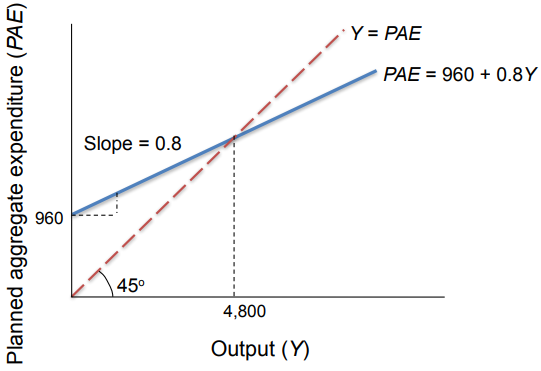
Short-Run Equilibrium

Short-run equilibrium is the level of output at which planned spending is equal to output

• No change in output as long as prices are constant

• Our equilibrium condition can be written Y = PAE

Output Greater then Equilibrium

Suppose output reaches 5,000 – Planned spending is less than output – Unplanned inventory increases – Businesses slow down production – Output goes down

Suppose output is only 4,500 – Planned spending is more than total output – Unplanned inventory decreases – Businesses speed up production – Output goes up

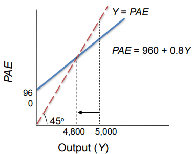
Income-Expenditure Multiplier

shows the effect of a one-unit increase in autonomous expenditure on short-run equilibrium output

• Initial planned expenditure = 960 + 0.8Y

• New planned expenditure = 950 + 0.8Y

  • The 10-unit drop in C implied a 10 unit drop in autonomous expenditure

  • Equilibrium changed from $4,800 to $4,750

  • A $10 change in autonomous expenditures caused a $50 change in output

  • Multiplier = 5

• The larger the mpc, the greater the multiplier

Stabilisation Policy

Government policies that are used to affect planned aggregate expenditure, with the objective of eliminating output gaps

• Expansionary policies increase planned expenditure

• Contractionary policies decrease planned expenditure

• Fiscal policy uses changes in government spending, transfers, or taxes

• Monetary policy uses changes in the money supply

The Role of Fiscal Policy

Tools of fiscal policy

• Government spending - Direct effect on PAE

• Taxation - Indirect effect on PAE

• Transfer payments - Indirect effect on PAE

Discretionary fiscal policy

• Government decisions to change:

  • Government spending (G) - Direct effect on PAE

  • Net taxes (T) - Indirect effect on PAE

• Both change the government deficit (G – T)

Government Spending

• Government spending is part of planned spending

  • Changes in government spending will directly affect planned aggregate expenditures

• Suppose planned spending decreases $10 from Y = 960 + 0.8Y to Y = 950 + 0.8Y

  • Equilibrium Y decreases from $4,800 to $4,750

    • Recessionary gap is $50

• Stabilization policy indicates a $10 increase in government spending will restore the economy to Y* at $4,800

US Military Spending

• Military spending as a share of GDP decreased sharply after World War II

  • Peaks for wars and Reagan military buildup

• Added demand from military spending helped end the Great Depression

  • Recessions associated with declines in military spending

  • Increases in G can help stimulate the economy

Crowding-Out Effect

• The tendency of an increase in government expenditure to increase the rate of interest, and reduce consumption and investment by the private sector

• Occurs when PAE is affected by changes in interest rates

The strength of the crowding-out effect depends on:

1. The responsiveness of consumption and investment to interest rate changes

   • For any given interest rate the crowding-out will be stronger the greater the resulting decline in consumption and investment

2. The responsiveness of the demand for money to interest rate changes

Taxes and Transfers

• Net tax (T) = total taxes – transfer payments – government interest payments

• Planned aggregate expenditures are influenced by changing total taxes and/or transfer payments

  • The effect is indirect, channelled through the effects on disposable income

    • Lower taxes or higher transfers increase disposable income

    • Increases in disposable income lead to higher C

Supply-Side Effects of Fiscal Policy

• Fiscal policy may affect potential output as well as potential spending

  • Investment in infrastructure increases Y*

  • Taxes and transfers affect incentives and can change potential output, Y*

• Supply-side economists emphasize the supply-side effects of fiscal policy

• Current thinking is more moderate

  • Demand-side effects of spending matter

  • Supply-side effects also matter

Fiscal Policy and Deficit Spending

• Government deficit is the difference between government spending and net taxes, (G – T)

  • Large and persistent budget deficits reduce national saving

  • Less saving means less investment which means less growth

• Managing the impact of the deficit limits the government's ability to use fiscal policy as a stimulus

  • Political considerations make it difficult to use contractionary fiscal policy

Fiscal Policy Flexibility

Two limits to fiscal policy flexibility

• The legislative process requires time

  • Change in fiscal policy may be slow

• Competing political objectives

  • National defence

  • Entitlements such as Medicare and income support

Fiscal Policy can be Effective

• Automatic stabilizers increase government spending or decrease taxes when real output declines

  • Built into laws so no decision is required

  • Unemployment compensation, progressive income tax

• Fiscal policy may be useful to address prolonged periods of recession

  • Monetary policy is more often used to stabilize the economy

Automatic Stabilisers

Automatic changes in the government budget deficit which help to dampen fluctuations in economic activity