hj

about 68% of the values fall within

one standard deviation of the mean

about 95% of the values fall

within two standard deviations of the mean

and about 99.7% of the values fall

within three standard deviations of the mean.

Normal Model

The model for symmetric, bell-shaped, unimodal histograms is called

How to represent a Normal Model

write N(μ,σ), with mean μ and standard deviation σ.

standard Normal model or the standard Normal distribution

The model with a mean of 0 and a standard deviation of 1 is called what, it is used with standardized z - scores

•Normal probabilities

•When the standardized value does not, we can look it up in a table of Normal percentiles.

•When the standardized value falls exactly 0, 1, 2, or 3 standard deviations from the mean, we can use the 68-95-99.7% rule to determine Normal probabilities

Tables

•use the standard Normal model, so we’ll have to convert our data to z-scores before using the table.

•These days, we can also find probabilities associated with z-scores use technology like calculators, statistical software, and websites.

statistical analysis

we often aim to estimate the true proportion of an event within a population.

Unfortunately, we usually cannot directly observe this true proportion.

To work with this concept, we'll label the true proportion as 'p.’

P-hat" (  ) is a common notation used in statistics to represent the sample proportion. It is used to estimate the true population proportion (p) based on data collected from a sample.

only two possible outcomes for an event

label one of them “success” and the other “failure.”

In a simulation

we set the true proportion of successes to a known value, draw random samples, and then recorded the sample proportion of successes.

sampling distribution

the distribution of proportions over many independent samples from the same population is called the sampling distribution of the proportions

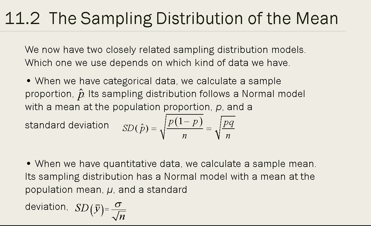
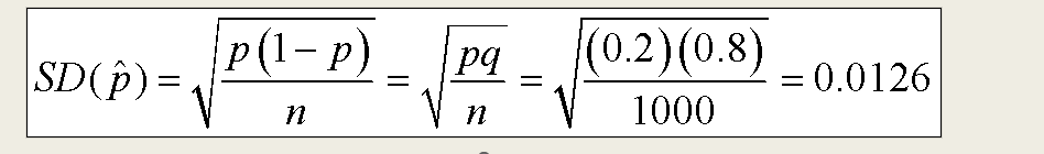
For distributions that are bell-shaped and centered at the true proportion, p, we can use the sample size n to find the standard deviation of the sampling distribution:

sampling error, and sampling cariability

that the difference between sample proportions referred to as sampling error is not really an error: It’s just the variability you’d expect to see from one sample to another. A better term might be sampling variability.

Standard Deviation (SD)

–measures the dispersion or spread of a dataset.

–It tells you how individual data points vary from the mean (average) of the dataset.

–It is used to describe the variability or the "average" distance between each data point and the mean.

–It's often used in descriptive statistics to understand the distribution of a dataset.

Standard Error(SE)

–is a measure of the precision of a sample statistic (e.g., sample mean or sample proportion) as an estimate of the population parameter (e.g., population mean or population proportion).

–It provides a sense of how much the sample statistic is expected to vary from one sample to another.

–Standard Error takes into account both the variation within the sample and the sample size.

How good is the Normal Model

For samples of size 1 or 2, the Normal model is not a good fit for representing the sampling distribution of proportions.

However, when we consider larger samples, the histograms of sample proportions become remarkably close to a Normal distribution.

As the sample size increases, the Normal model increasingly approximates the distribution of sample proportions, making it a better representation.

Central Limit Theorem(CLT)

The CLT states that for a sufficiently large sample size, the distribution of the sample means (or proportions) will be approximately normally distributed, regardless of the shape of the original population distribution, This holds true for a wide range of real-world scenarios.

Independence Assumption

The sampled values must be independent of each other.

–In statistical sampling, it's crucial that each observation is not influenced by or related to the others within the sample.

The Sample Size Assumption

The sample size (n) must be sufficiently large.

–A larger sample size often ensures that the results are more representative of the population.

The Randomization Condition

If your data come from an experiment, subjects should have been randomly assigned to treatments.

–For survey data, the sample should be a simple random sample of the population.

–Ensure that the sampling method was unbiased and the data are representative of the population.

The 10% Condition

If sampling was conducted without replacement, the sample size (n) should be no larger than 10% of the population.

–This condition ensures that the impact of sampling on the population is minimal.

The Success/Failure Condition

The sample size must be sufficiently large so that both the number of "successes," np, and "failures," nq, are expected to be at least 10.

–In our bank example, we observed 211 customers who defaulted (successes) and 789 who did not (failures). Both counts are at least 10, meeting this condition

What Can We Say about a Proportion?

1)“42.0% of all U.S. adults thought the economy was improving.”

•There is no way to be sure that the population proportion is the same as the sample proportion.

●

2)“It is probably true that 42.0% of all U.S. adults thought the economy was improving.”

•We can be pretty certain that whatever the true proportion is, it’s probably not exactly 42.0%.

3)“We don’t know the exact proportion of U.S. adults who thought the economy was improving but we know it is between 40.4% and 43.6%.” We can’t know for sure what the true proportion is in this interval.

●

4)“We don’t know the exact proportion of U.S. adults who thought the economy was improving but the interval from 40.4% to 43.6% probably contains the true proportion.” This is close to correct, but what is meant by probably?

An appropriate interpretation of our confidence interval would be:

“We are 95% confident that between 40.4% and 43.6% of U.S. adults thought the economy was improving.”

Statements like this are called confidence intervals.

The confidence interval calculated and interpreted here is an example of a one-proportion z-interval.

What does it mean when we say we have 95% confidence that our interval contains the true proportion?

Our uncertainty lies in whether our specific sample is one of the successful ones or one of the 5% that fail to produce an interval that captures the true value.

Sample proportions vary from sample to sample. If other pollsters collected samples, their confidence intervals would be centered around the proportions they observed.

What Does “95% Confidence” Really Mean?

§While we can never be absolutely certain that our confidence interval contains the true population proportion, the Normal model provides an important guarantee.

§The Normal model assures us that, on average, 95% of all theoretically possible intervals are "winners," meaning they cover the true population value.

§Conversely, only about 5% of these intervals miss the target.

§This is why we can confidently say that we are 95% sure that our interval is one of the "winners.”

When interpreting intervals, it's crucial to communicate precisely this level of confidence.

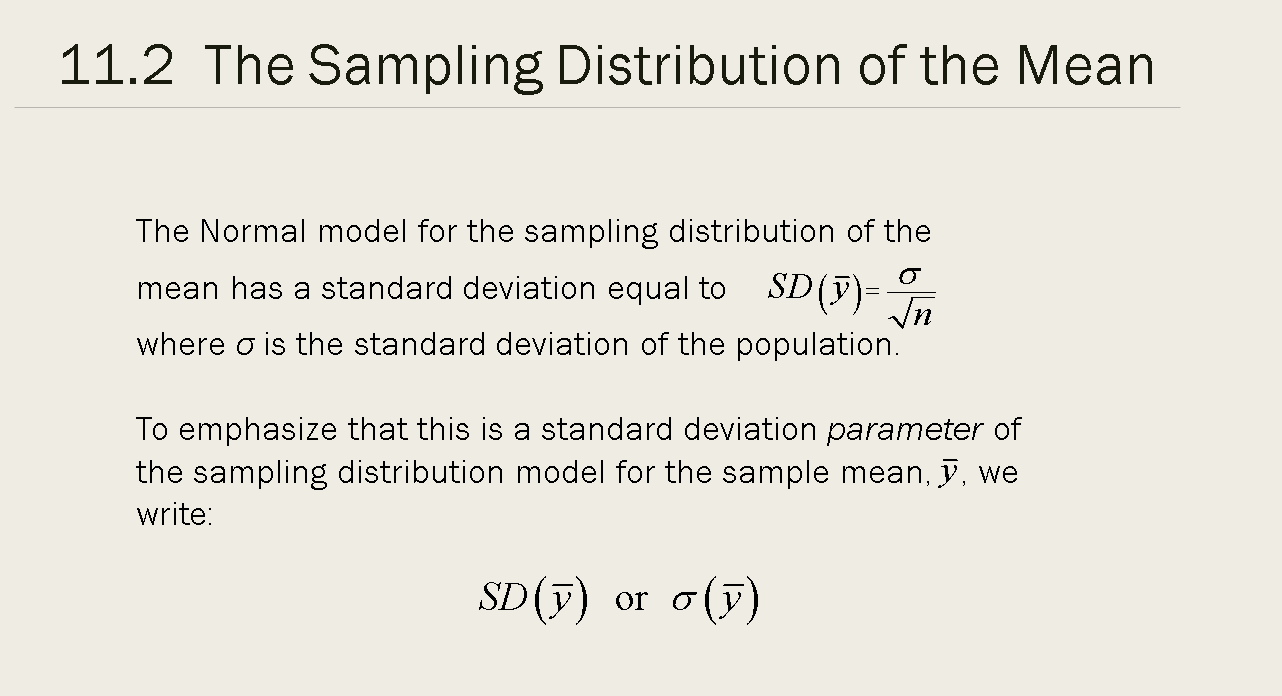
The Central Limit Theorem

Central Limit Theorem (CLT): The sampling distribution of any mean becomes Normal as the sample size grows.

This is true regardless of the shape of the population distribution!

However, if the population distribution is very skewed, it may take a sample size of dozens or even hundreds of observations for the Normal model to work well.