1042 BIOSTAT W4-

What are Confidence Intervals (CI)?

• A sample statistic is rarely the same as the parameter

• A difference between the sample statistic and the parameter may occur purely by chance or sampling variability

• So it is sensible to estimate the parameter by an interval centred on the sample statistic

• This interval is called the confidence interval

• Most should include the population mean

• Usually use a 95% level of confidence (sometimes 90% or 99%)

How can we use CI to tell the significance of data?

• If the confidence interval includes zero, the difference is not significant, otherwise the difference is significant, as the diagram below demonstrates

QS: The width of a confidence interval can be reduced without reduction of confidence level by decreasing the sample size

• FALSE

• If the sample size increases, the standard error decreases which results in a narrower confidence interval
  
  

How to calculate Confidence Intervals?

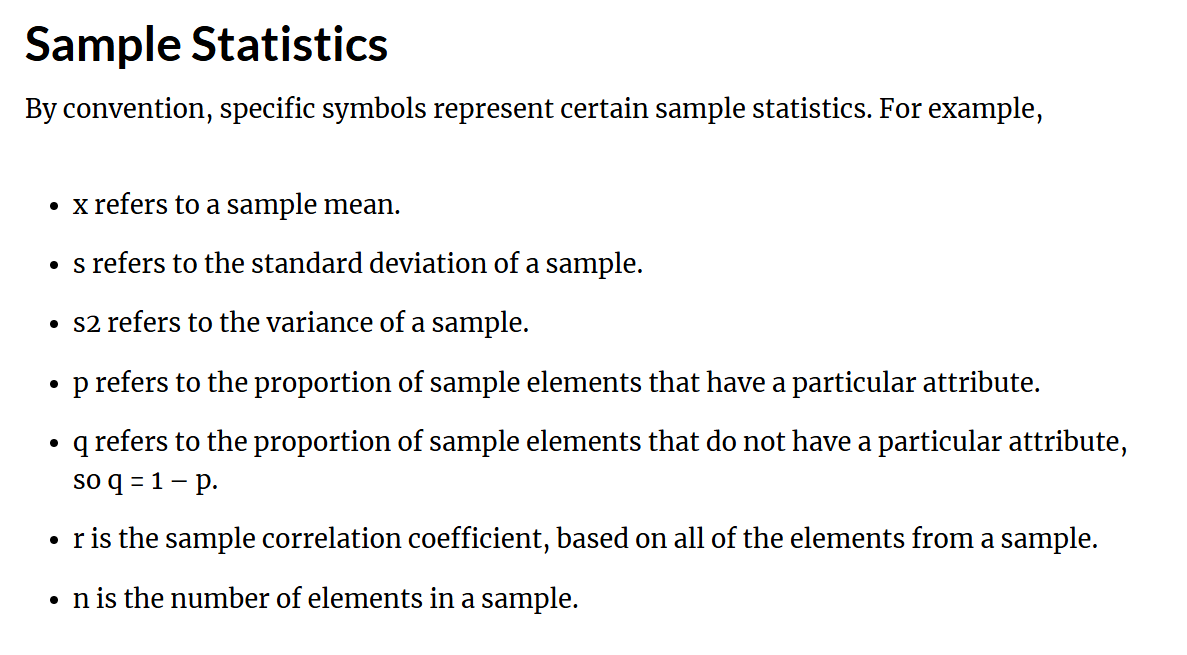
What are Sample Statistics?

What is Hypothesis testing?

• Hypothesis: A statement about the study population. We use sample statistics to make inferences about the population of interest

• We use statistical methods to analyse if the results observed in the sample are due to chance, or if there is actually a difference

• Why?

  • Sometimes an observed raw difference between groups turns out to be not an actual difference after considering all the evidence (e.g. mean difference, standard error)

• Allows us to analyse the results of studies

What are the 2 types of Statistical Hypothesis?

• Two‐sided hypothesis (common)

  • Null hypothesis: No difference between groups. (the same)

    • H₀: Population mean 1 – Population mean 2 = 0. (H₀: µ₁ ‐ µ₂ = 0)

  • Alternative: There is a difference between groups. (difference)

    • H_a: Population mean 1 – Population mean 2 ≠ 0. (H_a: µ₁ ‐ µ₂ ≠ 0)

• One‐sided hypothesis (less common)

  • E.g. Null hypothesis: Population mean 1 ≥ Population mean 2

    • Alternative: Population mean 1 < Population mean 2

  • OR Null: Population mean 1 ≤ Population mean 2

    • Alternative: Population mean 1 > Population mean 2

• Note: The Alternative (a difference) is what you want to “prove”

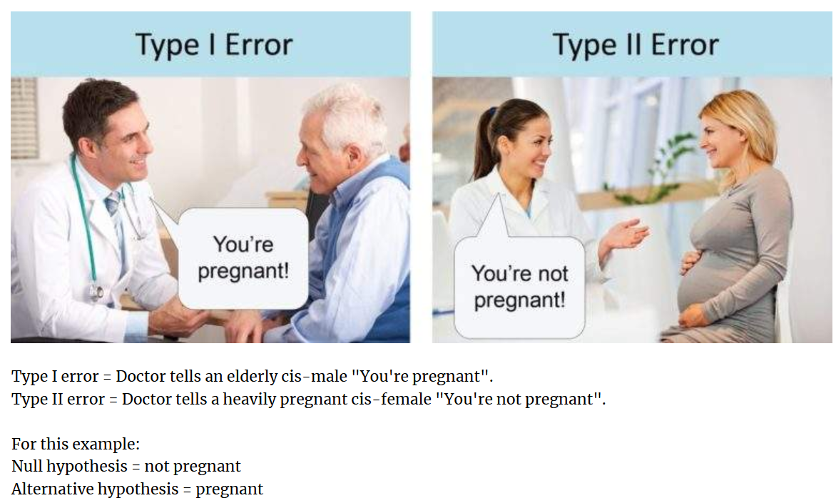
What is Type I and Type II error?

• We don’t know the true state of the null hypothesis – True / False

• We assume the null hypothesis is true (so no difference) and then we evaluate it from the sample data

• Conclusions from the sample data are affected by sampling variation

• Type I error = We reject the null hypothesis when the null hypothesis is true

• Type II error = We retain the null hypothesis when the null hypothesis is false

Null Hypothesis and the 2 types of Error example: Boy who cried wolf

Remember:

• Null hypothesis: No difference between groups. (the same)

  • H₀: Population mean 1 – Population mean 2 = 0. (H₀: µ₁ ‐ µ₂ = 0)

• Alternative: There is a difference between groups. (difference)

  • H_a: Population mean 1 – Population mean 2 ≠ 0. (H_a: µ₁ ‐ µ₂ ≠ 0)

Therefore our H₀ is that there is NO wolf. So Type I error occurs, when the true state of the Null hypothesis is TRUE (e.g. there is no wolf) but we reject the null hypothesis (thus we think there IS a wolf).

What is the usual value for a “p-value”?

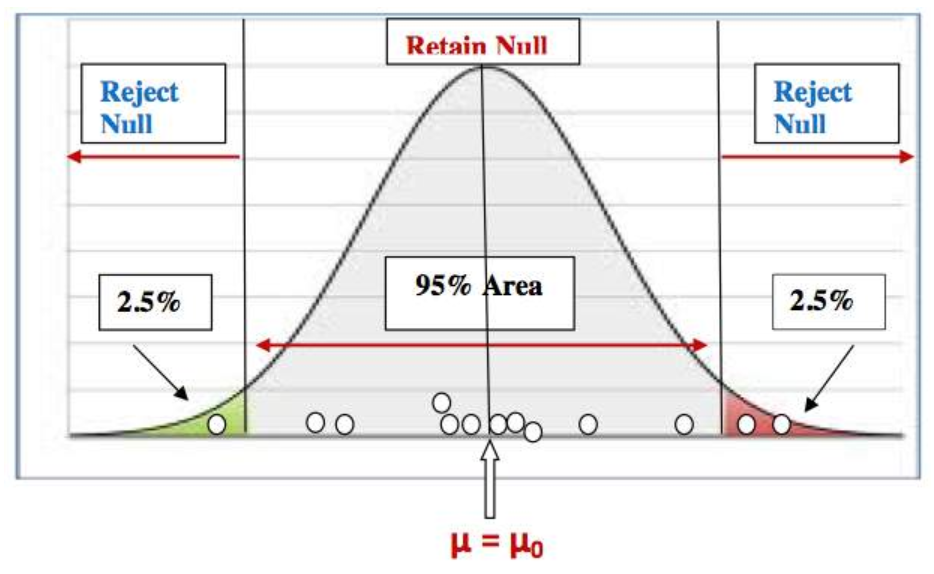
• The p‐value is normally 0.05. (Fits with 95% CI.)

  • This is the probability of a “Type I” error occurring

• If the p‐value > 0.05

  • Insufficient evidence to reject the null hypothesis

  • Thus “do not reject” or “retain” the null hypothesis

  • DO NOT say “accept” the null hypothesis!!

  • If the sample mean falls within 95% of the middle area, then we say that it is close to the population mean under the null and any differences between sample mean and null hypothesized population mean is due to sampling variability or by chance

• If the p‐value < 0.05

  • The probability that an observed result of big (or more) occurring due to chance is small

  • Thus sufficient evidence to reject the null hypothesis

  • We reject the null hypothesis (no difference), and accept the alternative hypothesis (there is a difference)

  • If the sample mean falls either in the lower 2.5% area or in the upper 2.5% area, then we say that the sample mean is so far out that a sample mean this large would rarely occur just by chance when the null is true

  • So we will conclude that the sample data does not support the null hypothesis and we go with the alternative hypothesis

Hypothesis Tests - What do P-values even mean?

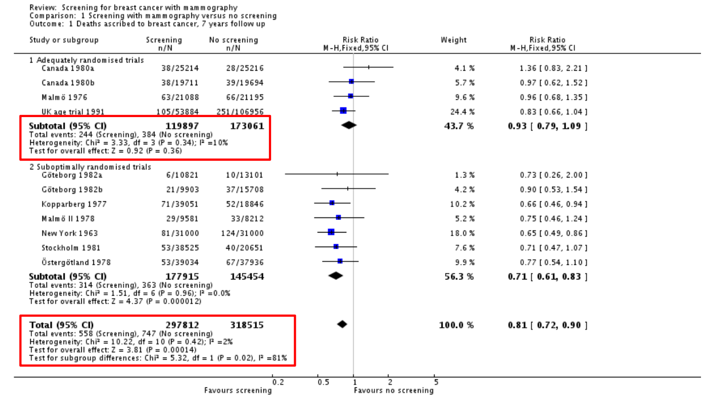
• Adequately randomised trials, p = 0.36

  • 36 out of 100 times, an observed effect being this big or more, is due to sampling variability or by chance

• Overall effect, p = 0.00014

  • 14 out of 100,000 times, an observed effect this big or more, is due to sampling variability or by chance

  • This means there is more likely to be a true difference

  • The study result is so rare that a chance factor can be ignored for the difference from the hypothesized value

What are the steps in Hypothesis testing?

• State the study

  • Summarise the study objectives (its importance and implications in public health)

  • State the study type

  • Write down the information you have (sample size etc.)

• 1) State the hypotheses

  • Null (no diff), Alt (diff). One or two‐sided? Justify

  • justify your selection of alternative hypothesis

    • For example, if you are considering a two-sided alternative hypothesis, provide evidence that supports your choice

• 2) State the assumptions & check them

  • Data should follow at least approximately normal

  • Patients in the sample should be selected randomly

  • Patients within a sample should not be related (or should be independent)

• 3) Analyse the data

  • Use the most statistical method to evaluate the hypothesis

  • Obtain the Test statistic value & p‐value (manual or software)

  • Calculate the 95% confidence interval too

• 4) Discuss the results & make an inference on the population

  • Discuss the summary statistics

  • Are the results significant or not?

  • Make an inference/conclusion on the study population

What are the types of tests (means)?

• One‐sample mean

  • Rare test in “real life” research

  • This is when you test one sample’s mean against a mean that you think it will be

• Difference between means

  • Large samples or known population SDs

  • Its rare the population SD is known and the mean is not!

  • Small samples, equal SDs — Far more common

  • Small samples, unequal SDs

• Mean of differences

  • Paired measurements

What are the 3 methods to test whether the SD is equal or unequal?

The formulas for SE and df for “difference of two means” is different for equal and unequal SDs

Method 1: Present the data graphically (histogram or boxplot)

• Compare the dispersion (spread) of the two groups

• If the spread of the data in each group is similar, assume equal SDs

Method 2: Calculate the ratio of the variances

• Note: Variance = SD²

• If the ratio < 2, assume equal SD

• If ratio ≥ 2, assume unequal SD

• Formula is the image

Method 3: Use a statistical package

• Use a hypothesis test procedure known as the Levene’s test for testing the null hypothesis that the groups have equal variances against the alternative hypothesis that the groups have unequal variances

• If the resulting p-value ≤ 0.05, reject the null hypothesis, i.e., consider unequal variances.

• On the other hand, if the p-value > 0.05, retain the null hypothesis, i.e., consider equal variances.

Is the population SD known or unknown and finding the p-value

Testing for equal or unequal SD → Method 3: Use a Statistical package

• Graph Pad Prism (and other stats packages) assesses whether the SDs are equal or unequal as part of the analysis process

• Hypotheses associated with this check:

  • H₀: The two groups are equal SDs

  • H_a: The two groups have unequal (different) SDs

• How to interpret the results:

  • If the p‐value > 0.05, we do not reject the null hypothesis (i.e. We assume equal variances)

  • If the p‐value < 0.05, we reject the null hypothesis. (i.e. We assume unequal variances)

Wording:

• “The results are statistically significant” – when the p-value < significance level

• “The results are not statistically significant” – when the p-value > significance level

How to determine what type of tests to do?

Example 1: Birth Weights → Step 0: State the Study

• The birth weights of children born to 14 heavy smokers and 15 non‐smokers were compared. The sample was from live births at a large teaching hospital

• What type of study design?

  • Cross‐sectional if “snap shot” in time

  • Cohort if mothers followed up and birthweights of their child collected later

• Data available:

  • Birth weights born to heavy smokers

  • Birth weights born to non‐smokers

  • Birth weight is continuous

Example 1: Birth Weights → What Test to use? And is the variance equal?

• “Independent” → can a mum be a smoker and non-smoker at the same time => NO, thus independent

Example 1: Birth Weights → Steps 1 Hypothesis & Step 2 Assumptions

• Null hypothesis: The population mean birth weight of babies born to heavy smokers and non‐smokers are the same

• Alternative hypothesis: The population mean birth weight of babies born to heavy smokers and non‐smokers is different

• Assumptions:

  • The two groups (heavy and non‐smoking) are independent

  • The mothers within each group are independent

  • The birth weight in each group follows a normal distribution (need to do the test - here we will just assume it is normal)

Example 1: Birth Weights → Step 3 Calculations

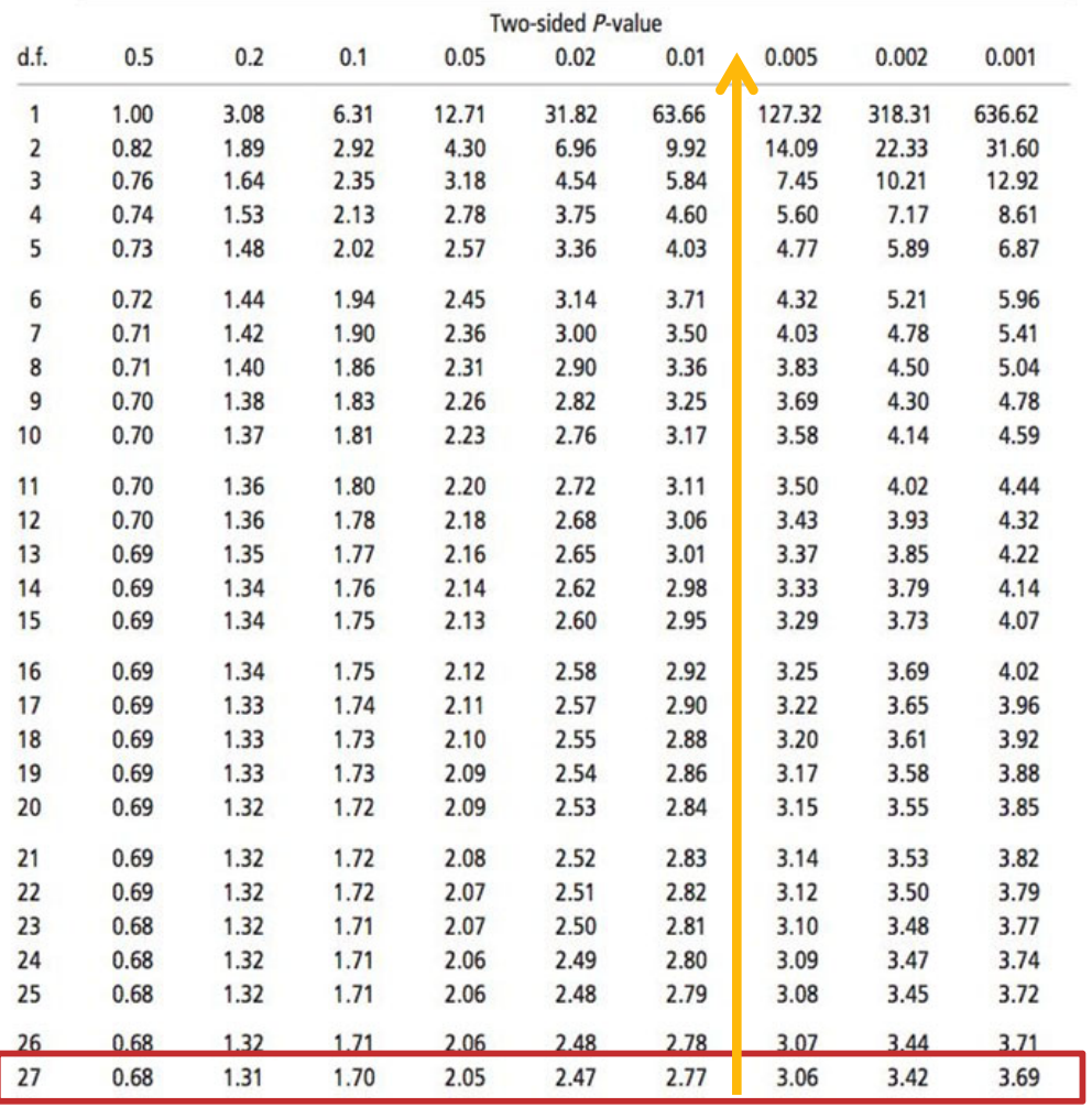
• Collate the information you have (image above)

• Calculations needed for the hypothesis test and 95% CI as followed in the image below

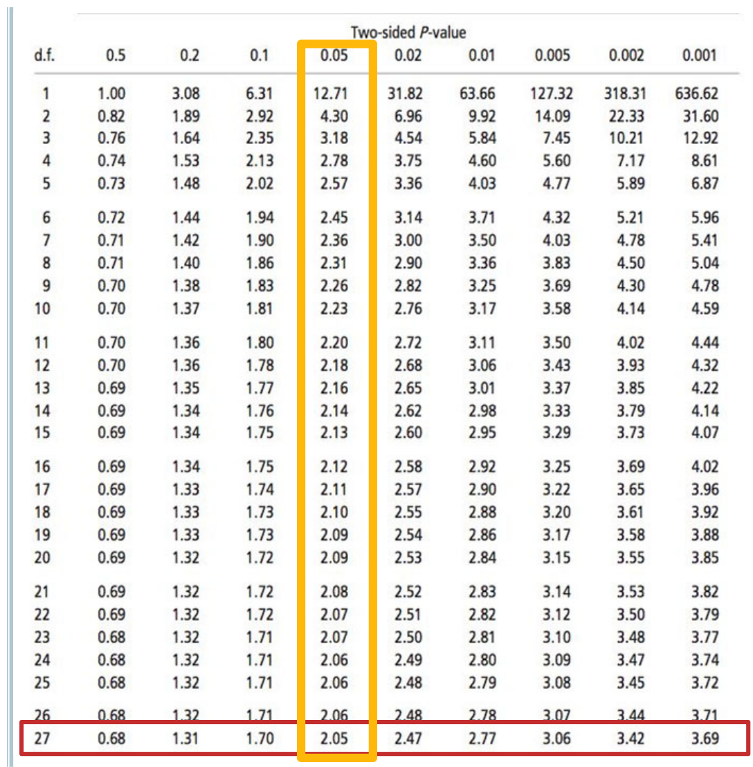
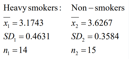
Example 1: Birth Weights → How to calculate T-multiplier?

• df = 14 + 15 - 2 = 27

• 95% CI means two-sided p-value is 0.05 (depicted in image above - two sides of the curve with 2.5%)

• T mult = 2.05

Example 1: Birth Weights → Calculate SE

Example 1: Birth Weights → Calculate the T-statistic

• Unpaired t-test → Independent t-test

• Look at 2-sided p-value

Example 1: Birth Weights → Calculate the p-value

• t‐statistic: ‐2.95

• p‐value is between 0.005 and 0.01

  • Note: A range is acceptable

  • A precise p‐value is obtained using a statistical package (see stats package videos for details)

• Interpretation:

  • The p‐value (between 0.005 and 0.01) is less than 0.05

• Decision:

  • Reject the null hypothesis (no difference)

  • Accept the alternative (there is a difference)

Example 1: Birth Weights → Calculate the CI

• We are 95% confident that the population mean difference between the birth weight of babies born to heavy smokers and non‐smokers falls between ‐0.77 and ‐0.14 kg

Example 1: Birth Weights → Step 4: Conclusion

• Report the means

  • The mean birth weight of babies born to smokers was 3.17 (± 0.46) kg and the mean of those born to non smokers was 3.63 (± 0.36) kg

• Report the CI and p‐value and comment on significance of the difference

  • The mean difference of ‐0.45 kg (95% CI of ‐0.77 kg to ‐0.14 kg [excludes 0]) and p‐value (between 0.005 and 0.01 [p‐value < 0.05]) allows us to reject the null hypothesis, providing evidence that the difference between groups is significant.

• Concluding remark giving the direction of difference

  • Hence babies born to mothers who smoked during pregnancy may have a reduced birth weight compared to those whose mothers did not smoke in the population

*In the end you should be able to write the conclusion without any headings

How to do the Two-Sample T-test for Unequal Variance?

What is the difference between T-multiplier and T-Stat?

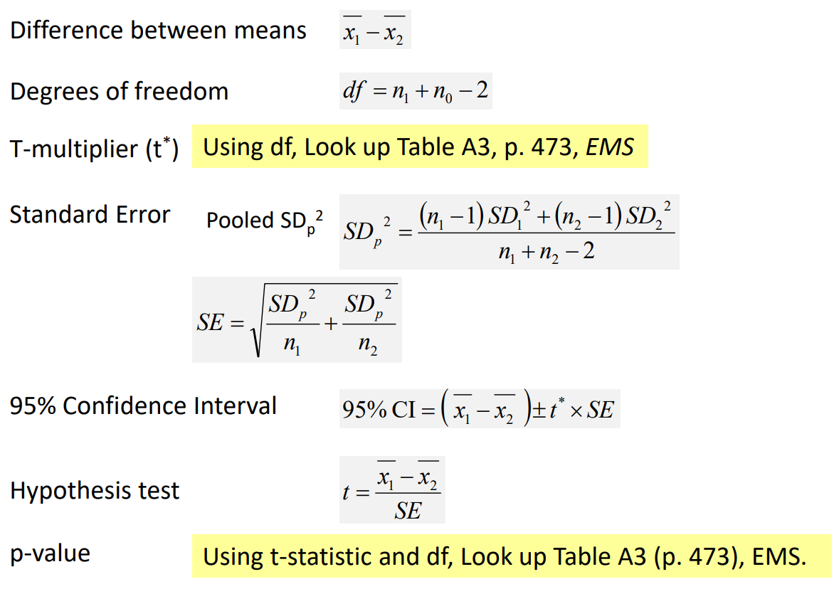
Formula for an INDEPENDENT T-test - EQUAL SD

Formula for an DEPENDENT paired t-test

Formula for an INDEPENDENT T-test - UNEQUAL SD

DEPENDENT Test example: Step 1 - Determine test

Consider the results of a clinical trial to test the effectiveness of a sleeping drug in which the sleep of 10 patients was observed during one night with the drug and one night with the placebo. The results are shown in the following table. Compare sleeping hours b/w the 2 groups.

What study designs use OR and RR?

• OR → When we start with the outcome

• RR → When we start with the exposure

• The RR (Relative Risk), is appropriate for cross-sectional, sample survey, randomised clinical trials, and cohort studies (prospective and historical)

• The OR (Odds Ratio), is appropriate for retrospective studies only. For example, case-control studies where the disease status is known but factors related to the disease are unknown.

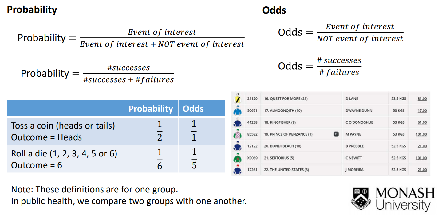
Probability vs Odds: What’s the difference?

What is the Relative Risk (RR)?

• Relative Risk = probability

• Compares risk of outcome in exposed compared to unexposed

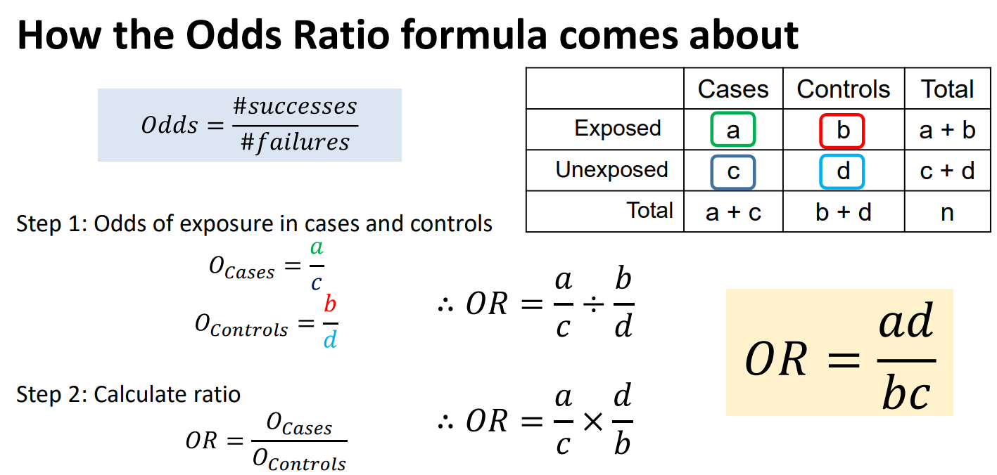
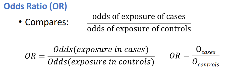
What is the Odds Ratio (OR)?

• Odds Ratio = odds

• Compared odds of exposure in cases compared to controls

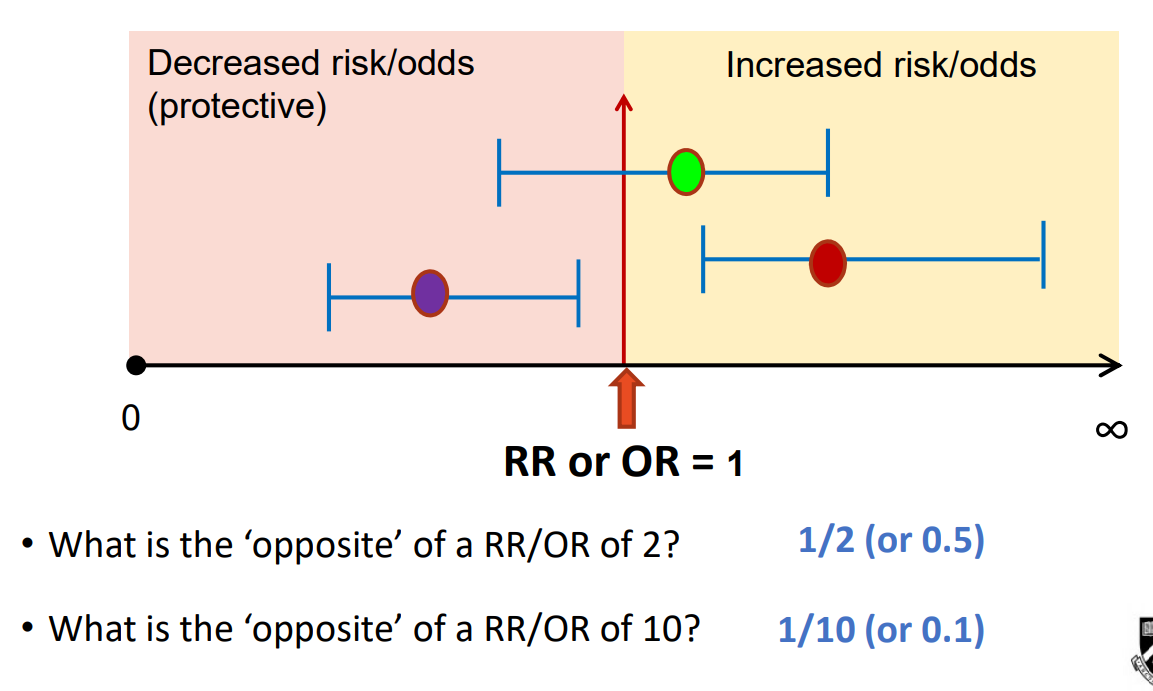
Are RR and OR normally distributed?

• When the RR or OR is equal t 1, that means there is no difference

• If RR or OR > 1 → means the exposure increases the outcome, so there increased risk

• If RR or OR < 1 → protective factor

Relationship between OR and ln(OR) (or RR and ln(RR)?

Confidence Intervals – data transformation (OR and RR)

• RR or OR: Not normally distributed

• lnRR or lnOR: Normally distributed

Logarithms and exponentials – quick explanation

Formulas for RR – calculating 95 % CI and p-value

• 1) Calculate RR

• 2) Convert to natural logarithm (ln) level

• 3) Calculate 95 % CI at ln level

• 4) Exponentiate to get back to RR level

Formulas for OR – calculating 95 % CI and p-value

• 1) Calculate OR

• 2) Convert to natural logarithm (ln) level

• 3) Calculate 95 % CI at ln level

• 4) Exponentiate to get back to OR level