L04 - Data Preparation and Preprocessing

Data Preparation

• Raw data is usually not directly suitable for modeling → it must be processed first.

• This is the most time-consuming stage in data mining (50%–70%).

• Goal: Prepare the final dataset for modeling.

• Data preparation ↔ modeling is usually an iterative process.

Data preparation types

• Data Construction: Create new attributes (e.g., derive new columns from existing ones).

• Data Reduction: Remove irrelevant features and keep the most important ones.

• Data Transformation: Reformat data (e.g., convert text-stored numbers to numeric type).

• Data Selection & Integration: Select the datasets to use, combine data from multiple sources.

• Data Cleaning: Fix or remove incorrect, missing, or noisy data.

Data Cleaning

Measurement errors

There are various types of measurement errors that can be addressed by data cleaning

• Missing values

• False or inconsistent data

• Noisy data

• Outliers

Handling Missing & False Data
What are the strategies for that? and what are the pros and cons?

• Delete data subset

  • Advantage: Simple, does not distort the data structure

  • Disadvantage: May cause loss of data

• Fill in / correct the value

  • Advantage: No data is lost

  • Disadvantage: May introduce bias

How can false / missing values be replaced?

Problem with false and missing values:

and two imputation concepts?

• Problem: True value is usually unknown, filling is based on assumptions.

• Mean / Median imputation:

  • Simple and fast.

  • Fill missing values with the mean or median of the variable.

  • Disadvantage: Introduces bias toward the middle of the normal range.

• Nearest neighbor imputation:

  • Replace missing values with values from the nearest neighbor.

  • More complex, may bias results toward existing examples.

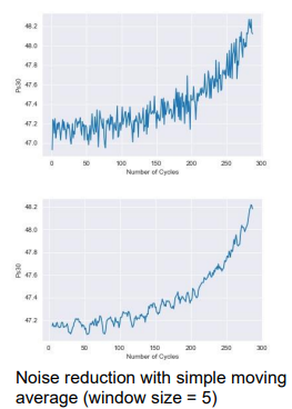
Noise'

Noise reduction can be done by what?

Noise is a random error or variance in a measured sensor signal.

Reduction method: Filtering

• Low-pass filter: Passes low-frequency signals, removes high-frequency noise.

• Simple moving average (SMA): Average of the last k data points.

Outliers

Data point far away from normal behavior.
Can distort data and cause wrong results.

• If true event → keep it.

• If measurement error → remove it.

Handling Outliers

• True outlier:

  • May represent extraordinary events (e.g., bird strike in an aircraft engine).

  • May be part of normal variability.

  • Should remain in the dataset.

• Measurement errors:

  • Outliers caused by measurement errors or wrong entries.

  • Should be treated like false values (cleaned or removed).

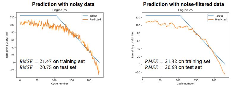
Noise filtering

• Noise filtering does not significantly change the average accuracy (RMSE).

• But it reduces random fluctuations in predictions → useful for practical application.

Scaling

• Many algorithms are sensitive to data scale:

  • Gradient descent algorithms

  • Distance-based algorithms (clustering, KNN)

• Different scales can cause unequal influence of features on the model.

• Solution: Transform variables so they vary over the same range.

Normalization & Standardization

• Normalization:

  • Transforms data to a range ([a,b], usually [0,1]).

  • Sets min value to 0, max value to 1.

  • Suitable for non-Gaussian distributions when min & max are known.

• Standardization:

  • Transforms data to have mean 0 and standard deviation 1.

  • Suitable for normally distributed data, resistant to outliers.

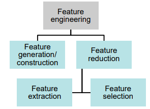
Feature Engineering

Feature engineering describes the whole process of creating, handling and selecting features that can be used for the next steps in a structured process.

• Create, modify, and choose features for modeling.

Feature engineering types and their definitions

• Feature generation/construction is the process of generating features from the preprocessed raw data by using common mathematical procedures like time-series analysis or frequency-domain analysis.
  Generation: Make new features from raw data (e.g., time-series, frequency).

• Feature reduction overarches the feature selection and feature extraction method with the goal to reduce the number of features in the database to those that contain meaningful information.
  Reduction: Keep only important features (selection + extraction).

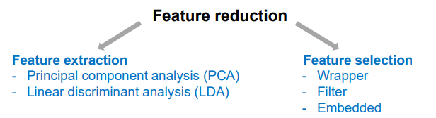
Feature reduction types

• Feature extraction: Extract meaningful features using transformation and aggregation methods (e.g., PCA, LDA).

• Feature selection: Select a subset of meaningful features (e.g., wrapper, filter, embedded).

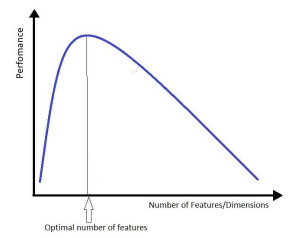
What is the Motivation for Feature Reduction?

• As dimensionality increases, data becomes sparse (curse of dimensionality).

• With a fixed number of samples, model performance can deteriorate.

• Data points required for good performance grow exponentially with more dimensions.

• More dimensions → data sparse.

• Same samples → worse performance.

• Need exponentially more data for good results.

What are the Feature Subset Selection Approaches?

• Filter: Uses statistical methods to judge feature importance (e.g., variance, correlation).

• Wrapper: Tests different feature combinations against an error function.

• Embedded: Combines model training with feature selection.

Feature Selection – Filter Methods

• Evaluate features using statistical tests (correlation coefficient, chi-square test).

• Input–output relationship:

  • Select best features for predicting output,

  • remove irrelevant ones.

• Input–input relationship:

  • Remove redundant features.

• Note: The k best attributes are not always the best k attributes together.

Feature Selection – Wrapper Methods

• Forward Search: Starts with an empty set, adds features one by one to find the best set.

• Backward Search: Starts with all features, removes them one by one to find the best set.

• Can be more accurate, but takes more computation time than filter methods.

Embedded Feature Selection

• Some ML algorithms perform feature selection during training.

• Lasso regression: Sets coefficients of unimportant features to 0.

• Decision tree: Most important features are at the top of the tree.

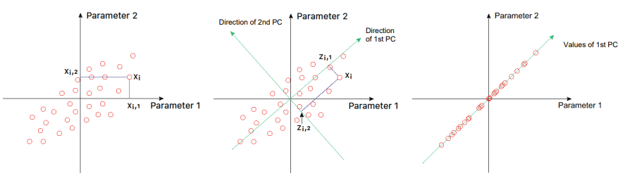
Principial Component Analysis

A Principial Component Analysis performs a linear orthogonal transformation of the data space to maximize the variance of the data along the first axis (principal component).

• PCA doesn’t reduce features by itself, but you can keep only components explaining most variance.

• Usually keep components explaining 70–90% of variance.

• Alternative: Kaiser criterion → keep components with eigenvalue > 1.

PCA - Definition and Summary

• PCA transforms data orthogonally into a new coordinate system, capturing maximum variance.

• Popular for dimensionality reduction.

• PC1 explains the largest variance.

• Can reduce noise, irrelevant information, and outlier effects.

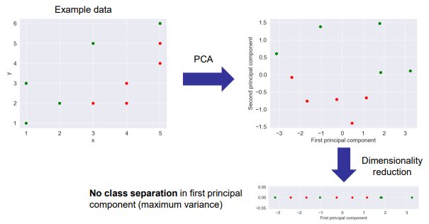
PCA – Classification example

• PCA maximizes variance, but not always good for class separation.

• In the example, two classes (red-green) remain mixed after PCA.

• In such cases, LDA (Linear Discriminant Analysis) might be better.

Linear discriminant analysis

Fisher‘s linear discriminant

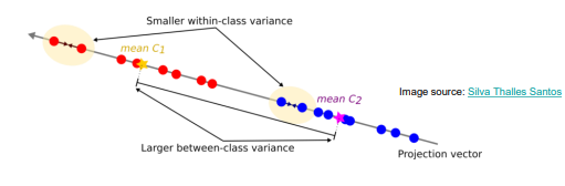
The main idea of a linear discriminant analysis in binary classification is to project the data to the one-dimensional line where classes are best separated.
Find the projection that best separates the classes.

LDA (Linear Discriminant Analysis)

How to find the optimal projection?

• Goal: Find the projection that best separates the classes.

• Two criteria:

  1. Large distance between class means (between-class variance).

  2. Small spread within each class (within-class variance).

• Maximize: (Difference of class means)² / (Total within-class variance).

• For n classes, dimensions can be reduced to at most n-1

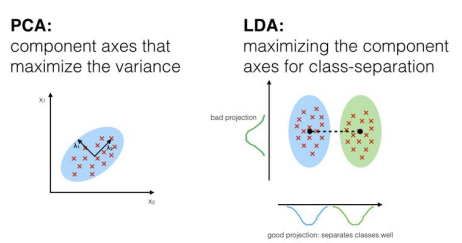
PCA vs LDA

• PCA:

  • Unsupervised

  • Can be used for any problem

  • Maximizes variance

  • Does not directly reduce dimension, can use variance threshold

• LDA:

  • Supervised

  • Only for classification

  • Maximizes class separation

  • Reduces dimension to at most n-1 for n classes

Feature Generation – Include Historical Information

• Goal: Create new features with extra information.

• Idea: Compare current sensor values to the initial (healthy engine) state.

• Calculate meanand standard deviation of first 30 cycles.

• Result: Significant improvement in prediction performance.

Feature Generation – Polynomial Features

• Goal: Create new features with additional information.

• Idea: Capture non-linear relationships between input features and RUL.

• Calculate all feature combinations with a polynomial degree of 2.

• Number of features increases from 24 to 325.

• Result: Large improvement in training set, but overfitting occurs.

• Solution: Apply dimensionality reduction in the next step.