fluid transport KNW3

ideal immiscible displacement conditions

• ignore finite solubility of the different fluid phases in e/o

• ignore compresibility of the displacing & displace fluid phase

fractional flow

the relative flow velocity of water with respect to the total flow velocity

mass flux, M

mass change in volume element & time interval

fluid phase velocity

the fractional flow functional value divided by the phase saturation because the true interstitial velocity depends on the volume occupied by the fluid phase, which scales with the phase saturation

steady state system

• both fluid phase velocities are adjusted to the same fractional flow point

• const Sw

front velocity

the velocity of the saturation change

fractional flow discriminations

• consider a monotonic behavior of the saturation profile

• apply the material balance a second time

• assume shock front formation.

shock

a mathematical description of the motion of a surface of discontinuity

shock waves

the properties of a surface of discontinuity of a solution of a first-order quasi-linear hyperbolic system of partial differential equations.

what do we use shock waves

• “shocks” are observed in numerical simulations

• shocks are typical problems arising in the context of first-order quasi-linear hyperbolic partial differential equations e.g. MBE

wave classification

depending on their spreading character

• Spreading waves: wave becomes more diffuse on propagation (non-sharpening)

• Sharpening waves: wave is self sharpening and becomes less diffuse →the wave will become a shock, even if the initial condition is diffuse

• Mixed waves: Like the Buckley-Leverett wave

• Indifferent waves: neither spreading nor sharpening – might appear as shocks in the absence of dissipation

heat capacity

the heat that is required to change the temperature by ∆T

thermal diffusivity

measures the ability of a material to conduct thermal energy relative to its ability to store thermal energy

heat equation

a parabolic partial differential equation that describes the sedistribution of heat (or variation in temperature) in a given region over time.

sensible heat

a change of temp of a substance l

latent heat

heat absorbed or released by a substance during a (first order) phase transition (e.g. transition of steam to liquid water) without a temperature change.

enthalpy

measure of the total energy of a thermodynamic system

cold water recharge

a doublet system with a hot producer and a cold re-injector, cold water is injected into:

• single phase liquid water region → pressure increase/ maintenance

• two-phase (steam-water) res → decreasing pressure due condensation & declining temp

• superheated steam zone → increase the pressure as long as no two-phase zone

forced convection = advection

fluid transported by external forces like applied pressure gradient

natural convection

convection is caused by intrinsic mechanisms like fluid density differences (maybe caused by a temperature gradient) in a gravity field

Rayleigh number, Ra

a dimensionless number describing the buoyancy driven flow

• Ra<Ra,c → heat transfer primarily by conduction

• Ra>Ra,c → heat transfer primarily by convection

effect of temp on crude oil

viscosity decreases w/ increasing temp → increasing mobility

mixing

a result of true physical effects & lack of info/ description

mixing types

• Diffusive mixing

• Microscopic dispersive mixing

• Macroscopic dispersive mixing

mass balance formula

change in fluid mass in volume, V = net fluid inflow across surface of V + net gain fro sinks & sources in V

fracture = crack

any mechanical discontinuity in a rock incl. joints & faults

joint

fracture that exhibits only a small opening displacement, usually less that the grain-size of the host rock

fault

fracture with measurable displacement parallel to surface

vein

fracture with a measurable opening that is filled with mineral, or igenous rock (dyke, sill or sheet).

fracture characteristics

• Orientations / sets

• Spacing, spacing distribution and clustering

• Length distribution

• Density / intensity

• Connectivity

• Fragmentation and matrix block size

percolation categories

• growth: disconnected → connected network

• addition: sub-critical, percolation threshold & super critical

reservoir processes

• unfrac. res: Predominantly forced processes → Tested by core floods

• frac. res: Predominantly spontaneous processes → tested by AMOTT type of experiment

how do we describe fracture networks

explicitly or statistical depending on:

• the typical length scale of the fracture or the fracture network

• our knowledge about the fracture system

• The available computational power.

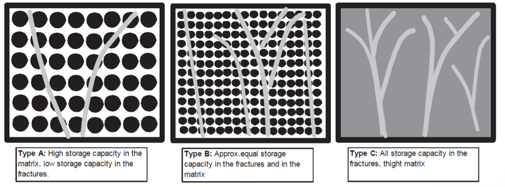
McNaughton classification of fracture networks

• type A: high storage capacity in the matrix & low storage capacity in fracture

• type B: approx. equal storage capacity in the matrix & fracture

• type C: all storage capacity in the fracture, tight matrix

nelson’s classification of fracture networks

• type I: feature provides the storage capacity & perm. → geothermal application = hot dry rock

• type II: matrix provides storage capacity & fracture provides the permeability → hydraulically stimulated res

• type III: fracture provides permeability assists, good matrix porosity & perm

• type IV: fracture creates anisotropy

fractured res characteristics

• High apparent permeability

• Early breakthrough of injected fluids or early gas/water coning

• Highly directional flow behavior (and localized in the producing interval)

• Large variability in well productivities and recoveries

• Permeability depends on stress and fluid pressure

fractured res uncertainties

• Productivity of wells and sustainability of rate

• In the case of injection: time to injectant breakthrough (oil or enthalpy production decline)

• Recovery mechanism controlling rate dependency

• Contacted reservoir volume → sweep effects

info sources

• Knowledge about the global geological setting

• Seismic survey

• Monitoring of seismic activities during well stimulation and well testing

Local information from wells:

• Borehole imaging

• Core analysis

• Flow monitoring

flow tests

• classical well test analysis

• steady state flow tests from injection to production well

fracture flow modelling difficulties

• the general lack of data

• bridging and extracting data taken at different length scales

• Integration of diverse data from different sources in a fracture network

• How to translate and simplify the reservoir model for efficient modeling?

network properties

• size and size distribution of the fractures

• number density of fractures

• orientation and connectivity

• aperture and related permeability and porosity

reservoir fracture models

• discrete fracture modelling

  • Deterministic discrete fracture models → Explicit representation of the fractures

  • Stochastic discrete fracture models:

    • Natural fractures

    • Position and orientation statistically distributes

    • Radii fractal distributed

    • Overlapping and activated apertures → permeability

• continuum models

dual continua approach assumptions

• Fracture permeability can be averaged

• All fractures are interconnected

• Each grid-block contains a statistically meaningful number of fractures

• Grid-block fracture properties can be averaged

• Matrix-block sizes are normally distributed so they can be averaged

• Grid-blocks are isometric (equal dimensions)

MINC method = multi interactive continua

1. Primary grid discretizing the reservoir volume

2. Secondary grid formed by nested sub-cells representing the matrix

3. Is able to handle the transient flow of heat and fluids between matrix and fractures numerically (in contrast to transfer function of DC models)

4. for multiphase flows, or coupled fluid and heat flows, transient periods can be very long → it is necessary to resolve the driving pressure, temperature, and mass fraction gradients at the matrix/fracture!

continuum scale consequences

• avg momentum → describes the macroscopic velocity field

• heat transfer → describing a random molecular movement w/ no net flux across a macroscopic interface

fick’s 1st law

Diffusive flux is proportional to the particle concentration gradient!

pure advection

keeps the shape of a concentration profile, but translates the center of mass (=flow)

pure diffusion

keeps the center of mass of the species, but eliminates concentration gradients (smearing out)

gas diffusion coefficient parameters

• temp

• pressure

• molecular weight

• molecular diameter

dissipative processes

• Molecular diffusion

• Electrochemical migration → diffusion of charged species induced by the electrical potential (driving force).

• Diffusion in concentrated solutions driven by the gradient of the chemical potential rather than by the concentration gradient.

dispersion

macriscopic process of spreading of mass from highly concentrated areas to less concentrated areas, depending on the heterogeneities in the flow path

dispersion types

• mechanical/ tailor → results for the fact that variations of the flow velocity exist not captured in advective transport witch only considered an average flow rate

• macro

• tortuosity

tailor dispersion process

in a capillary tube, the flow close to the tube wall is slower than in the center → leads to a velocity distribution and hence to a smearing of the tracer (solute) front.

why is tortousity length squared?

affects the flow twice

• the velocity

• driving force

microscopic dispersion

• Molecular diffusion – related to the thermal motion of molecules – independent of advective processes.

• Mechanical dispersion (velocity distribution) due to the flow profile in a single capillary (Poiseuille profile).

• Dispersion by tortuosity due to pathways of different

  length within an REV of porous media flow.

mobility

• 𝑴 > 𝟏: unfavorable → high-K is invaded more easily and flow resistance is decreasing with time → displacement is unstable.

• 𝑴 < 𝟏: favorable mobility ratio → high perm layer initially invaded faster than low permeable layers, but flow in high-K slows down with time due to increasing resistance to flow.