1BB3 Macroeconomics Final Exam Study

Covers all information from chapter 4-12 VIDEOS ONLY

Chapter 4: GDP

• Market value of all final goods and services produced in a region in a given period during a year

• Measures of how much stuff a country produces

• Based off market value

• Only legal things considered in this metric

• Attempts to capture all things produced

• Only accounts for final goods, this avoids double counitng

Chapter 4: Forms of GDP calculation

Income method: Adds incomes earned from production.

Expenditure method: Adds spending on final goods and services.

Chapter 4: GDP calculation, expenditure method

Y=C+I+G+NX 

Adds

• C consumption

• I investment

• G government spending

• NX exports minus imports

To find

• Y, total GDP

Chapter 4: Housing in the GDP

• New housing included as investment spending the year it is built because it lasts a very long time and provides a flow of services each year

• Sale of an existing home is NOT included as part of GDP, this just transfers asset nothing new is made

Chapter 4: Rent vs Owner in GDP

• Both provide services to families

• Both are included in consumption services

• Owner occupied housing is a rare example of something included in GDP even if there is no market transaction, owner operated housing is included by estimated rental value

Chapter 4: Gross National Income (GNI) & Gross National Product (GNP)

• Market value of all final goods and services produced by a country’s factors in given period

• To be included in Canadian GNP, the factors of production used to make good or service must be Canadian owned

• GNI and GNP are the same thing

Chapter 4: GDP vs GNI

Ford makes a car in Oakville that costs 30k 

• 20k is cost of labor 

• 10k is profit to ford 

• Canadian GDP increases by 30k, but GNI is only increased by 20k (labor cost) 

GDP includes all goods or services produced in Canada

GNI includes all goods and services produced with Canadian owned factors of production, regardless of where it takes place

Chapter 4: GDP theory

• Calculated by adding up price times quantity over all goods and services produced each year

• GDP rises if prices rise or if we make more

Chapter 4: Nominal vs Real GDP

• By holding prices constant in some “base” year and re calculating GDP, we arrive at real GDP

• Once we have nominal GDP and real GDP, we can use these to calculate the overall price level in an economy

Chapter 4: GDP Deflator

• Measure of the price level

• Nominal GDP divided by Real GDP times 100

• Inflation rate is the percentage change in the price level from one year to the next

Chapter 5: How unemployment is determined (CONCEPT)

• Stats Canada divides the working non institutional civilian adult population into 3 mutually exclusive categories

• Determined by phone survey

• Unemployed is when you have no job BUT are looking for work

Chapter 5: Calculations related to employment/unemployment

• Unemployment rate is the number of unemployed divided by labor force times 100

• Labor force participation rate is labor force divided by adult population times 100

• Employment rate is number of employed divided by adult population times 100

Employment rate is NOT equal to 100 minus the unemployment rate because of division factor

Chapter 5: Circle example of categorizing Canadians

Imagine the whole population as one big circle for this explanation

• Outermost circle, whole population

• Then one layer in is the adult population (15+)

• Then another layer in is the non institutional civilian adult population (does not include prisoners, military, or hospital workers)

• In the non institutional civilian adult population circle it gets split into three, employed, unemployed, and not in labor force

Chapter 5: Unemployment compensation

• Benefits paid to workers who find themselves unemployed

• Reduces the negative impact on family income in case of unemployment

• Increases the opportunity cost of going to work

Cost of working:

• Direct cost (lunch out, parking, gas)

• Opportunity cost (not collecting E.I)

Chapter 5: Unemployment diagram

• E.I Shifts the labor supply curve left changing equilibrium

• Minimum wage above equilibrium wage is binding, market is not in equilibrium, but this is justified and reasoned which is why its done

• Labor market: Firms are buyers, workers are sellers

Chapter 5: Calculating CPI

• Consumer Price Index, measures the overall cost of goods and services for typical Canadian households

• Begins calculation by deciding which goods are included in the “basket” then they find the cost of it

• CPI is the cost in current year divided by cost in base year times 100

• CPI is a measure of the overall price level of economy

• Most used price index for reporting the inflation rate, the rate of change of the price level from one year to next

Chapter 5: Inflation with CPI

Inflation rate = (CPI this year − CPI last year) ÷ CPI last year × 100

Chapter 5: CPI vs GDP Deflator

• Both measure of the price level

• Different “basket of goods”, the GDP deflator is all goods produced in Canada while the CPI is all goods bought by typical households

Chapter 5: Unanticipated inflation example

• Mortgage is a loan on a house, bank agrees on interest rate and loan term

• Real interest rate is nominal interest rate minus inflation rate

• A problem with unanticipated inflation is the unexpected transfer of wealth between borrowers and lenders

• Inflation greater than expected, wealth moves from lenders to borrowers

• Inflation less than expected, wealth moves from borrowers to lenders

Chapter 6: Per capita GDP, is it accurate for what we use it for?

• Accounts for all goods and services produced in country

• Higher per capita GDP typically means other development metrics improve

• Used to see how a country is evolving over time

• GDP per capita = GDP ÷ population

• To find year over year do ((future-initial)/initial)x100

Chapter 6: Calculating average annual growth rate over a period

AAGR = (growth rate year 1 + growth rate year 2 + …) ÷ number of year

Chapter 6: Rule of 70

• How many years does it take for real GDP per capita to double

• Calculated by dividing 70 by growth rate in order to find doubling time

Chapter 6: Sources of growth

• Labor productivity: Output per worker or hour worked

• Increasing capital: Each worker hour has more access to capital to produce

• Technological improvements: Directly increases output per worker for given amount of capital

• Property rights: Ensures private firms are more likely to invest in a company converting to extra money for growth

Chapter 6: Closed economy GDP calculation

Y=C+I+G

• No NX term here, so this must be a _____ economy

Chapter 6: Types of savings

• Savings by households are private savings

• S to p (private savings) = Y+TR-T-C

  • Earned income plus transfer payments minus taxes and collections

• S to g (government/public savings) = T-TR-G

  • Taxes collected minus transfer payments minus government spending

Chapter 6: Government budget position

• Budget surplus if T>G+TR

• Budget deficit if T<G+TR

• Government debt is an accumulation of past deficits

T = Taxes…G = Gov spending…TR = Transfer payments

Chapter 6: National income accounting identity

• Y=C+I+G same as I=Y-C-G

• Definition of savings is private and public combined

  • National savings equals investment, found through algebra

  • Typically, only equal in closed economy

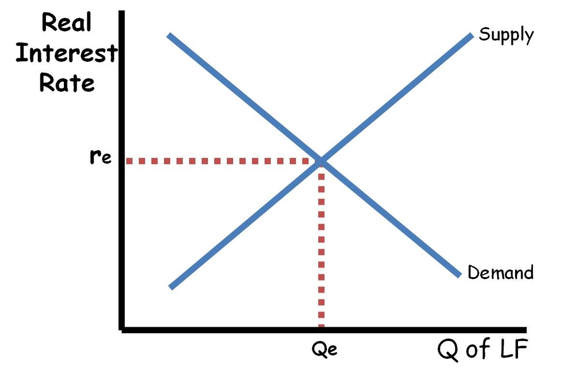
Chapter 6: Loanable funds diagram model

• Supply and demand for loanable funds brings savers and borrowers together

• Axis: Real interest rate on vertical axis and quantity of loanable funds on horizontal axis (measured in dollars)

Chapter 6: Reality vs course assumption

• Reality: Households, governments, and firms all both borrow and save

• Course assumption: All borrowing is done by firms who want to invest and all savings are done by households and governments whose income is greater than their current spending

• For simplicity treat government borrowing as negative savings (makes model easier to understand)

Chapter 6: Demand for LF

• Firms borrow to invest (purchase new capital)

• Slope: higher interest rates means higher cost of borrowing, negative relationship between interest rate and investment (demand for LF)

• Shift factors:

  • When firms need/want to purchase more capital at any given interest rate, demand for LF increases

  • When firms need/want to purchase less capital at any given interest rate, demand for LF decreases

Chapter 6: Supply for LF

• Households and governments save when their inflow of funds is greater than their spending, they supply this saving to the market for LF

• Slope:

  • Household’s, at higher interest rates, holding everything else constant, more savings now leads to higher consumption later… higher interest rates households are incentivized to save more

  • Positive sloped S curve due to private savings

  • Governments, no relationship between public savings and interest rate

• Shift factors:

  • When households/governments save more at any given interest rate, supply of LF increases 

  • When households/governments save less at any given interest rate, supply of LF decreases 

Chapter 6: Market for LF diagram

Chapter 6: Analyzing and understanding shocks

Example 1 

• Uncertainty about the future causes firms to decrease investment in capital goods, demand curve shift left, if increase shift right 

• Look at vertical axis to see interest rate 

• Look at horizontal axis to see investment spending, ivestment spending equal to saving 

• Private savings go down because lower interest rate indicates so 

• Public savings feels no effect if focus is on firms 

Example 2 

• The government decreases spending, holding taxes and transfers constant, this moves supply right due to government savings increasing  

Remember that when one curve shifts, there is always movement along the other curve, it is HIGHLY unlikely both will move from one factor

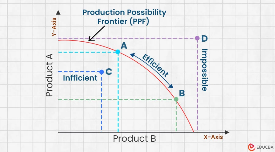
Chapter 7: Economic growth in the PPF diagram

(Production Possibility Frontier)

• PPF: Consumer/capital goods diagram

• Capital goods are machinery and robots, things used this year to produce goods and services

• Technological growth pushes out PPF curve outwards

• Closer to left of graph is more consumer goods, closer to right is more capital goods

• This graph shows where society chooses to dedicate our production/consumption, this will affect the next year

• Todays decisions affect tommorow’s possibilies

Chapter 7: PPF diagram

Chapter 7: Productivity

• The quantity of goods and services a worker can produce in an hour

• This is determined by physical capital, natural resources, human capital, and technological knowledge

• Production function shows how we combine inputs to produce products

Chapter 7: Production function formula

Y = A x F(K,L,H,N)

• Y is output 

• A is technology 

• K is physical capital 

• L is labor 

• H is human capital 

• N is natural resources 

Chapter 7: Return to scale

• If all inputs double, output doubles. Constant returns to scale.
  If output more than doubles, increasing returns to scale.
  If output less than doubles, decreasing returns to scale.

• For simplicity of course we will assume constant returns to scale

Chapter 7: Marginal product

• Product = output

• Marginal = extra

• Marginal product is output produced with one extra unit of an input

• Diminishing marginal product means the additional output produced by adding an extra unit of labor (19th unit) is smaller than the additional output produced by the unit of labor before (18th unit) (this explains the shape of the PPF diagram)

Chapter 7: Production function and policy

• Anything that increases on the left side of equation raises left side

• Policies

  • Protecting intellectual property incentive to increase A

  • Support of R&D incentive increases A

  • Subsidizing education increases in H or L

Chapter 8: Aggregate expenditure

• Total planned spending on final goods and services in an economy

• AE = C + I + G + NX

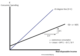
Chapter 8: Consumption

• Spending by households on goods and services

• Consumption function is the relationship between consumption and income

• Marginal propensity to consume (MPC) is the fraction of change in income that is spent on consumption… slope of the consumption function

Chapter 8: Consumption function

• Disposable income on horizontal axis and consumption spending on vertical axis

• Vertical intercept dictates the piece of consumption that does not depend on disposable income

• Things that shift curve up or down is net wealth, price level, interest rate, expectations

• Consumption is positively related to disposable income

• MPC tells us how much households increase consumption in response to 1 dollar increase in disposable income

Chapter 8: Consumption function diagram

Chapter 8: Aggregate expenditure simple model

• Shows spending at various levels of GDP for a given price level where spending is given by C+I+G+NX

• In equilibrium Y=AE

Chapter 8: Aggregate expenditure = real GDP

• Horizontal is real GDP and aggregate expenditure is vertical

• Will only be equal to real GDP at one value, at intercept

• Output is the 45-degree line, if AE is higher or lower over time the gap will close until equilibrium is reached

Chapter 8: Conclusion thoughts

• Inventories are the adjustment mechanism when spending does not equal output 

• If spending is higher than output inventories must be drawn down in order to fill the spending orders 

• If spending is lower than output inventories build up 

Chapter 8: Autonomous spending

Planned spending independent of current income or GDP, determined by firms, government, or foreign buyers, such as investment, government purchases, and exports.

Chapter 8: Simple spending multiplier

• Found by doing 1/(1-MPC)

• When any autonomous component of spending rises by 1$, real GDP rises by multiplier

Chapter 8: Multiplier intuition

• The 1 dollar increase in spending causes household income to rise by 1 dollar, people increase both consumption and savings, the higher consumption spending causes a further increase in income

Chapter 8: Shifts in aggregate expenditure

If autonomous consumption, investment, government spending, or net exports change, the AE curve shifts.
Inventories adjust to the gap between output and spending.
Y changes until the economy returns to macro equilibrium.

Chapter 8: Spending Multiplier – Concept

A change in government spending (ΔG = change in G) triggers multiple rounds of income and consumption:

• Round 1: ΔG → initial increase in income

• Round 2: MPC × ΔG → households spend part of Round 1 income

• Round 3: MPC² × ΔG → households spend part of Round 2 income
  Total change in income: ΔY = ΔG (1 + MPC + MPC² + …)

Chapter 8: Spending Multiplier – Formula & Reason

Total change in income ÷ initial change in spending:
ΔY / ΔG = 1 / (1 − MPC)
Reason: Each round of spending triggers more consumption.
The repeated rounds form an infinite geometric series because MPC < 1.

Chapter 8: Using AE to derive AD

• Start with a point on AD (Y₁, P₁)

• If P rises, planned spending falls

• Drag a line down from AE equilibrium to see new Y

• Repeat to trace the AD curve

• AE diagram shows how changes in P affect Y and derive AD.

Chapter 8: Shifts in AD curve

• Begins with a point on the initial AD curve

• Suppose investment spending increases what happens to the AD curve

• Increase causes shift out this shift causes shift in the AD curve

Chapter 8: Calculating Y and MPC – Closed Economy Example

• Closed economy: NX = 0 → Y = C + I + G

• Example: Y = 30 + 0.8(Y + 20 − 30) + 35 + 40

• Simplify: Y = 105 + 0.8(Y − 10)

• Solve: Y − 0.8Y = 105 − 8 → 0.2Y = 97 → Y = 485

• MPC = 0.8 (from consumption function coefficient)

Chapter 8: Solving for Equilibrium Income (Y) – Concept

• Start with Y = C + I + G (closed economy).

• Plug in consumption as C = autonomous consumption + MPC × disposable income (Y − T + TR).

• Add autonomous investment (I) and government spending (G).

• Combine terms with Y on one side and constants on the other.

• Solve for Y: Y = total autonomous spending ÷ (1 − MPC).
  Key idea: The economy’s equilibrium income depends on total autonomous spending and how much households spend out of extra income (MPC).

Chapter 8: Consumption function deep dive

• Slope of consumption function is the MPC

• This function will shift if non income determinants of consumption change such as net wealth, price level, interest rate, expectations

• e.g of function C=30+0.8(Y+TR-T) *30 is y int and 0.8 is slope 

• Solve for C+I+G to find slope of AE

• Shifts in AD Curve:

• Begin with a point on the initial AD curve 

• Suppose autonomous consumption spending increases, what happens to the AD curve 

• MPC times the increase in Y int is the horizontal distance change 

Chapter 9: Overview

• Aggregate demand and aggregate supply model 

• Involves 3 curves 

• Need to understand how slopes are determined 

• Need to understand what causes shifts 

• 2 concepts of equilibrium 

• Automatic adjustment equilibrium 

• Many variables show up in this diagram 

• Real GDP and Price Level axis 

• Unemployment does not show up on diagram but it's a key part 

Chapter 9: Slope of AD

• The AD curve has a negative slope

  • Wealth effect, how consumption changes when price changes

  • Interest rate effect

  • International trade effect, deals with net export change to price lvl

  • Anything that causes any component on left side of Y=C+I+G+NX will cause curve to shift

Chapter 9: Aggregate Demand

• Demand has to do with buyers 

• We have an equation that divides real output (GDP = Y) into categories according to who purchases the goods Y=C+I+G+NX 

Chapter 9: Aggregate Supply

• Supply has to do with production

• Real GDP and price level from the production side of equation

• Long run = economic growth = production function

• Y= A*F (K, L, H, N) 

Chapter 9: Long Run Aggregate Supply

• Slope A, K, L, H, N do not depend on price 

• LRAS is vertical 

• Any change on left hand side variable will cause the LRAS curve to shift 

Chapter 9: Short Run Aggregate Supply

• In the long run, there is no relationship between P and Y on the supply slide, this is not true in the short run

• Reasons for a positive relationship between P and Y on the supply side

  • Sticky wages

  • Menu costs

• Shift factors

  • Short term supply shock

  • Expected price level

Chapter 9: Sticky wage theory

• Nominal wages are “sticky” they are fixed in the short run, flexible in the long run (firms and workers usually agree to contract with fixed time period)

• What firms and workers really care about is real wage, for firms when real wage rises they are worse off but workers are better off

Chapter 9: Real wages, Nominal wages, and “P”

Real wage = W ÷ P.

• W is nominal wage. P is price level.

• If P rises and W stays fixed, real wages fall.

• Lower real wages make labor cheaper.

• Firms hire more labor and produce more.

• Y rises.

Chapter 9: Equilibrium

• When SRAS and AD touch there is equilibrium

• When SRAS, AD, and LRAS touch there is long ruin equilibrium

• Long run equilibrium is also referred to as y hat, the potential real GDP

Chapter 9: Shocks on the AD AS model

AD

• Slope of AD curve has to do with how consumption, investment spending, and net exports change

• Increases in any components cause shift right, decrease causes shift left

AS

• Supply shock that effects inputs into production that we think are temporary will cause shift

• Oil cost can shift SRAS curve

• Expected price level causes shifts

Chapter 9: Definitions

• Recession, any time output is below potential (left side)

• Expansion, any time output is greater than potential (right side)

Chapter 9: Away for LR equilibrium

• If Y is below potential Y, economy is in recession which leads to unemployment rates being high which leads to excess labor supply which leads to workers willing to take lower wages which leads to production costs falling which leads to firms producing more which leads to SRAS shifts right

• If y is above potential Y economy is in expansion which leads to unemployment rates low which leads to excess labor demand which leads to firms paying more wages which leads to production costs rising which leads to firms producing less which leads to SRAS shifts left

• When economy not in LR equilibrium automatic function exists to push economy back to LR equilibrium

• This mechanism works through labor markets, SRAS curve will shift, restoring long run equilibrium 

Chapter 9: Dynamic AD AS Model

• Used to explain economic fluctuations and long run growth.

• Over time LRAS shifts right due to tech progress and growth in K and L.

• LRAS pulls SRAS right as capacity expands.

• Population and income growth raise C, I, and G.

• Higher spending shifts AD right over time.

Chapter 10: What is money

• Something that is regularly used to buy goods and services

• Money does not equal income or wealth

Chapter 10: Functions of money

• Must be a medium of exchange

• Must be a unit of account - how we measure prices

• Must store value - asset

• Standard of deferred payment

  • Standard of deferred payment means money is used to settle debts in the future.

Chapter 10: Money in the Canadian economy

• M=C+D

• C is the currency in the hands of the public, not money in vaults but with the public

• D is demand deposits, demand means payable on demand and is another term for chequing accounts

• Money is an asset that is regularly used to buy goods and services, this does not include credit cards

Chapter 10: Money creation

• Current banking system makes money come from thin air, this is because there are two main components to money, currency in hands of public and chequing accounts

• If money were just a commodity, then banks would not have the ability to create money

Chapter 10: Reserves

• Reserve ratio: the fraction of total deposits that the banking system holds in reserve

• Reserves: the currency held in the bank vault waiting to be taken out

• T account: Shows the total amount held at a point in time.
  The numbers are actual balances, not how much they changed. Changes get shown by updating the balances, not by adding plus or minus signs.

Chapter 10: Money multiplier

• The total amount of deposits the banking system generates with each dollar of reserves

• Calculated as 1/reserve ratio

Chapter 10: More about money and deposits

1st way of thinking

• How much does a bank need in reserve, if there is a given amount of deposits

2nd way of thinking

• How much can the bank loan out, and how much in deposits can it support, for a given amount of reserves

• Bank creates money through lending out excess deposits they take in

• Textbook explanation is unrealistic, banks do not call up loans they simply slow loaning rate till reserve is built up

Chapter 10: Monetary policy

• This is increasing and decreasing the money supply to achieve specific goals for economy

• Primary tool is the open market operations > buying (selling) government bonds/securities from (to) the public

(brackets is whats actually happening)

Chapter 10: Open market operations, sale and purchase

Purchase

• This causes bonds to go from public to BoC and then the bank gives people money, leads to increase in money supply

Sale
- This causes bonds to go from bank to public and then the people give the bank money, leads to decrease in money supply

Chapter 10: Interest rates

• Prime rate, overnight rate, policy interest rate, bank rate

• Prime rate is the commercial rate banks charge their best customers

• Overnight rate is the rate commercial banks charge each other for 24 hour loans

• Policy interest rate is the BoC target for overnight rate

• Bank rate is the rate BoC charges commercial banks

Chapter 10: Course assumption

• Assume the BoC can completely control money supply

• Reality is they can not because households have control as to how much they choose to save and commercial banks can choose to keep excess reserves

Chapter 10: Quantity theory of money

• The quantity of money in the economy determines the price level in the economy

• Rate of growth of the money supply determines the inflation rate in the economy

Chapter 10: Velocity

• Rate at which money changes hands/circulates

• Divide spending by amount of current to find velocity

Chapter 10: Quantity equation

• M*V=P*V

• M is money, V is velocity, P is price level, Y is real GDP, P*Y is nominal GDP

Chapter 10: Quantity equation growth rates

Product rule

Chapter 10: Price level

Price level is nominal GDP over real GDP

Chapter 10: Barter economies

• Double coincidence of wants – a major shortcoming of barter economies that for barter to occur, each person must want what the other person has 

Chapter 11: Income/Money “decision tree”

• Earn income (flow) 

  • Save 

    • Adds to wealth (stock) 

      • Financial assets 

        • Money 

        • Non-monetary assets (stocks, bonds, etc.) 

      • Physical assets 

• Consume 

As income goes down the flow everything else receives a bit of the flow 

Chapter 11: Money markets in the short run

• Assume that the economy has only two financial assets, money and bonds

• Assume that money does not pay interest, but bonds do pay interest

• Opportunity cost of money is the interest you could earn by financial wealth in the form of bonds

• At low interest rates, people hold more of their wealth as money, at high interest rate more is held in bonds

Chapter 11: Money market diagram

• Demand for money has negative slope, higher interest rate means less quantity of money demanded

• Money supply “set” by BoC (course assumption)

• Change in money demand affects interest rate

Chapter 11: Money market diagram shocks

• If income rises, consumption goes up which leads to money demanded curve shifting right

• If banks conduct open market sale of bonds, public purchases bonds with money, resulting in money supply curve shifting left

Chapter 11: Monetary policy

Recession

• High unemployment

• BoC wants to shift AD out to the right

Expansion

• Risk of coming inflation

• BoC wants to shift AD into the left

Chapter 11: Monetary policy diagram

• Supplying more money shifts AD curve right pulling out of recession

• Supplying less money shifts AD curve left slowing spending pulling out of hasty expansion

• Central banks want to help eliminate high unemployment and reduce risk of inflation

• Can use monetary policy to shift AD to restore LR equilibrium sooner than waiting for automatic mechanisms to kick in

Chapter 12: Fiscal policy

• Typically when we use this term we are referring to discretionary fiscal policy which is changes in government spending, taxes, or transfers designed to impact economic variables such as GDP, the unemployment rate, or the price level

• In recession use expansionary fiscal policy and in expansion use contractional fiscal policy

Chapter 12: Automatic Stabilizers

• “Automatic” in the sense that changes in taxes and transfers that kick in when income fluctuates

• When GDP falls, income taxes falls and transfers rise which leads to income falling by less than if these taxes and transfers were not in place, thus mitigating the swings in aggregate demand that result from economic shocks

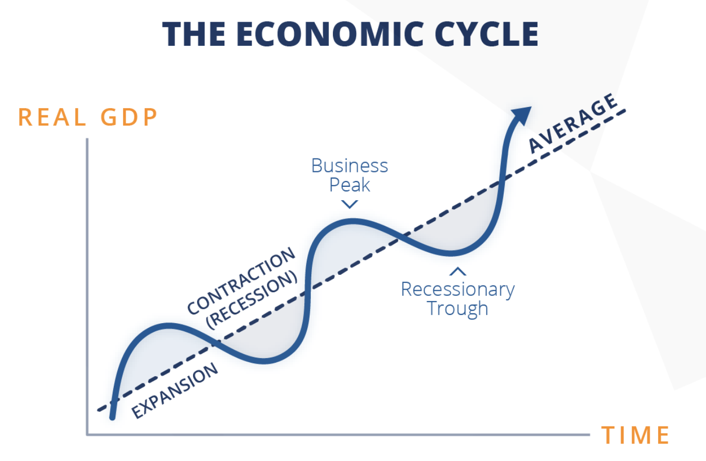
Chapter 12: Automatic stabilizers and the stylized business cycle

• Wavy line on a 45-degree line gets tighter because of automatic stabilizers

• Automatic stabilizers reduce fluctuations in AD

• Can see this in either the stylized business cycle diagram or AD-AS diagram

Chapter 12: Stylized business cycle diagram

Make note of PEAK and TROUGH placement

Chapter 12: Spending multiplier

• Simple Spending Multiplier = 1 / 1-MPC 

• When government spending rises by 1-dollar real GDP rises by SSM 

Chapter 12: Simple Spending Multiplier Intuition

The 1 dollar increase in spending causes household income to rise by 1 dollar; people increase both consumption and saving which leads to the higher consumption spending causes a further increase in income