MSE 3015 | Exam 1 Content

drift velocity (average velocity of charge carriers - electrons or holes - DUE to an electric field; likely why electric field is in the formula) = mobility (how easily the charge CARRIERS move through the material) times the electric field (force per unit charge acting ON the carriers)

J = current density [A/m2]

n = number of charge carriers per unit volume [1/m3]

e = charge of an electron [C]

v_d = drift velocity [m/s]

Memory: JEN Drives. J = E N V_d. Current density = charge of electron times number of electrons times drift velocity!

Units of Electrical Conductivity

1 / (ohm * m) = ( S / m)

Replay Formula

Units of Resistivity

ohm * m

Substitutional Alloy

An alloy (a material made by combining two or more elements, WHERE at least one is a metal) where atoms of one element replace atoms of another element in the crystal lattice!

Example: Brass!

Brass = Cu + Zn.

Some Zn atoms replace Cu atoms at regular Cu lattice sites. See left!

Because Zn and Cu atoms are similar in size, Zn can substitute for Cu without completely changing the crystal structure.

*Note: A substitutional alloy IS a type of solid solution!, specifically a substitutional solid solution!

Combined Matthiessen and Nordheim Rules

See left!

“resistivity of the matrix due to scattering from thermal vibration and other defects” => means the electrical resistivity of the main material (the matrix) comes from electrons being scattered by things that disturb their movement. Matrix = the continuous/main phase of the material!! Defects or other phases = things that disrupt the regular crystal structure, such as impurities, vacancies, OR particles of a second/larger phase!

Photovoltaic Effect

Chat: Def: Process where light energy is converted directly into electric energy. Simple Def = generation of electrical voltage/current when light is absorbed by a semiconductor. This is the principle behind solar cells.

Connection to Planck’s Equation. (See Left.). => So, the frequency (or wavelength of light determines the energy of each phonon, which affects whether the phonon can generate charge carriers in the solar cell.

Probability Primer

Sample space => all possible outcomes.

We shall denote a sample space by S, and define a random variable by the result of a rule (function) that associates a real number with each outcome in S. Random variable X → a rule that takes each outcome and assigns it a number. Meaning: XX takes an outcome from SS and gives you a real number. Example: Flip a coin twice. Sample space: S={HH,HT,TH,TT}S=\{HH,HT,TH,TT\}. Define a random variable XX = number of heads.

This paragraph is basically explaining what probability means and the 3 basic probability rules (axioms). Let's make it much easier. 1. Events AA and B. Remember: Sample space SS = all possible outcomes. Event AA = a group of outcomes we're interested in. Event BB = another group of outcomes. For example, rolling a die: S={1,2,3,4,5,6} Let A={rolling an even number}={2,4,6}. 2. What is P(A)P(A)? P(A)P(A) means the probability that event AA happens. There are two ways to think about it: Frequentist perspective:
"If I repeat the experiment many times, how often does AA happen?" Example: Roll a die 1,000 times. If you get a 1 about 167 times. P(1)≈1671000≈0.167P(1)\approx \frac{167}{1000}\approx0.167 which is close to 16.\frac16. Bayesian perspective:
"How likely do I think AA is to happen?" Axiom #1: Probability is between 0 and 1 0≤P(A)≤1\boxed{0\leq P(A)\leq1} Think:

• P(A)=0P(A)=0 → impossible

• P(A)=1P(A)=1 → certain

• P(A)=0.5P(A)=0.5 → 50% chance

Complement

The complement of AA, written AcA^c, means:

A does NOT happen.

Therefore:

P(Ac)=1−P(A)\boxed{P(A^c)=1-P(A)}

⚠ Your paragraph appears to have the equation reversed. It says P(A)=1−P(Ac)P(A)=1-P(A^c), which is also mathematically true, but the more common form is:

P(Ac)=1−P(A)\boxed{P(A^c)=1-P(A)}

Example:

If

P(A)=0.7P(A)=0.7

then

P(Ac)=1−0.7=0.3.

Axiom #2: The whole sample space has probability 1 P(S)=1\boxed{P(S)=1}

Why?

Because something in the sample space must happen.

For a die:

S={1,2,3,4,5,6}S=\{1,2,3,4,5,6\}

The probability of rolling some number from 1–6 is 100%:

P(S)=1.

Axiom #3: Non-overlapping outcomes add together

If events cannot happen at the same time, you can add their probabilities.

For example, on one roll of a die:

P(1)=16P(1)=\frac16

and

P(2)=16.P(2)=\frac16.

You cannot roll a 1 and 2 simultaneously.

Therefore:

P(1 or 2)=P(1)+P(2)=16+16=13.P(1\text{ or }2) = P(1)+P(2) = \frac16+\frac16 = \frac13. 🧠 Easy way to remember the 3 axioms

1 → Between 0 and 1

0≤P(A)≤10\le P(A)\le1

2 → Whole S = 1

P(S)=1P(S)=1

3 → No overlap = Add

P(A or B)=P(A)+P(B)P(A\text{ or }B)=P(A)+P(B)

So the big picture is:

Sample space S→events A,B→assign probabilities​

Probability Primer Cont.

Axiom #1: Probability is between 0 and 1. 0 <= P(A) <= 1.

Axiom #2: The whole sample space has probability 1 [Because something in the sample space must happen.]. P(S) = 1. [Text: The complement of A, Ac, is defined as all events in S that are not in A; P (A) = 1 − P (Ac)].

Axiom #3: Non-overlapping outcomes add together.

Discrete, random variables => a random variable that can take separate, countable numerical values. Two random variables X,YX,Y: Two different rules/numerical measurements applied to the same experiment.

P (A), can be viewed as the frequency of occurrence of the event (the “frequentist perspective”). Equivalently, P (A) represents the likelihood of the event occurring;

Probability Primer

Discrete random variables: use a PMF (Probability Mass Function; it gives the probability that a discrete random variable takes a particular value: P(X =x) which gives P(X=x) directly. For a fair die, P(X=6)=1/6. Continuous random variables: use a PDF, p(x). It gives probability DENSITY, not the probability that X=x. For an interval [a,a+da], P(a≤X≤a+da)=∫aa+dap(x) dx≈p(a) da. The total area under the PDF must equal 1: ∫−∞∞p(x) dx=1. Most importantly, for a continuous variable, P(X=a)=∫aap(x) dx=0. So p(a) is not the probability that X=a. It is the probability density at a. A higher p(a) means values near a are more likely, but any exact single point has probability zero.

For discrete random variables, we shall use probability mass functions (PMFs)!!
PMFs return a RETURN for the discrete random variable, X. For the unbiased six-side die. P (X = 6) = 1/6, etc. For CONTINUOUS variables, we shall use probability density functions (PDFs), denoted by p(x). [Chat: Discrete variable = can only take separate, countable values. Continuous variable = can take any value within a range, including decimals]. A PDF is related to a probability through an INTEGRAL relationship, which is unity over the whole sample space. For example, in one dimension, (−∞ < x < ∞) =

∫ ∞

−∞

p(x) dx = 1. The probability that x is between a and a + da is

P (a ≤ x ≤ a + da) =

∫ a+da

a

p(x) dx ≈ P (a) da (2)

Note that P (a ≤ x ≤ a+da) may be a very small number even at the “peak” of a distribution

if da is small; however, it will be larger than all others for similarly chosen da and different

1

x. Furthermore, it doesn’t really make sense to say that, “the probability of x = a is P(a)”

because as (2) shows, this limiting case gives P (x = a) =

∫ a

a

p(x) dx = 0.

Probability Primer Cont.

Define a random variable by the result of a rule (function) (= the equation that tells you what to do to an input to get the output) that associates a real number with each outcome in S. => A random variable is a FUNCTION/RULE that assigns a numerical value to every possible outcome of a random experiment. S = the sample space, meaning the set of all possible outcomes. A random variable X takes each outcome in S and assigns it a real number. Sample space is S = {1,2,3,4,5,6}. Define X as: X = the number that appears when the die is rolled. Ex. Outcome: 1 | X(outcome): 1; Outcome: 2 | X(outcome): 2, etc. HERE, X is a random variable because it assigns a number to each outcome. Another example: Suppose you flip two coins: S = {HH,HT, TH,TT}. Define X as: X = the number of heads. Then: X( HH) = 2, X( HT) = 1, X( TH) = 1, X(TT) = 0. NOTICE that the outcomes themselves are HH, HT, TH, TT, while the random variable converts those outcomes into numbers! In one sentence: A random variable is a rule that turns each possible outcome of a random experiment into a real number.

For simplicity, consider two discrete random variables that are associated with events in the sample space, A and B. => Ex. Roll a Die. Sample Space: S = {1,2,3,4,5,6}. Suppose: Event A = rolling an even number: A = {2,4,6}. Event B = rolling a number greater than 4: B = {5,6}. The textbook is basically saying: let's use two events, A and B, within the sample space, and study the probabilities associated with them. A and B are events, while random variables are numerical quantities associated with outcomes. So if your notes say “two discrete random variables associated with events A and B,” they may be simplifying the terminology. More precisely, A and B are events, not random variables themselves. Sample space → contains outcomes → events A/B are groups of outcomes → random variables assign numbers to outcomes.

The probability of A, denoted by P(A), can be viewed as the frequency of occurrence of the event (the “frequentist perspective”). Equivalently, P (A) represents the likelihood of the event occurring; this is called the “Bayesian perspective,” which will prove useful for interpreting conditional probability.

Probability axiom #1 states that P (A) is a real number between 0 and 1. The complement of A, Ac, is defined as all events in S that are not in A; P (A) = 1 − P (Ac). “Probability axiom #2” says that P(S) = 1. [Aka the frequency of the occurrence of S = 1; makes sense]. Probability axiom #3” will be defined below, but basically it says that if we have n outcomes that don’t overlap, the probability of all of them occurring is just the sum of the probabilities for each outcome!

For discrete random variables, we shall use probability mass functions (PMFs). => For a discrete [not decimal numbers], we use a PMF to describe the probability of each possible value. Think of a PMF as a table/rule that tells you how likely each outcome is. IF X is a discrete random variable, its PMF is: p_x(x) = P(X = x). PMF = the probability that X equals a particular value x. Ex: Rolling a dice: Let X = the number you roll. x = 1; P(X = x) = 1/6 | x = 2; P(X = x) = 1/6, etc. The PMF tells us: P(X=3) = 1/6. SO, the PMF gives the probability for each possible discrete value of X. Easy to remember: Discrete => PMF => Probability for each Point.

PMFs return a probability for the discrete random variable, X. For the unbiased [fair] 6-side die, P(X = 6) = 1/6, etc. For continuous variables!!, we shall use probability DENSITY functions (PDFs), denoted by p(x). PDF is related to a probability through an integral relationship, which is unity over the whole sample space [saw similar in notes for this unit!]. For example, in one dimension,

(Look to left!). [Integral from -inf to +inf of p(x) [aka the PDF] * dx] = 1.

Chat: For a continuous random variable, we use a PDF to describe how probability is distributed over possible values. For example, the probability that XX falls between aa and bb is: So the integral of the PDF over an interval gives the probability of being in that interval. What does “unity over the whole sample space” mean? Since something in the sample space has to happen, the total probability must equal 1:

AKA: PMF → Add probabilities. PDF → Integrate probabilities.

The probability that x is between a and a + da is: Look to the left! Reminder: P(..) = PDF!

More explanation on next card.

Probability Primer Cont.

The key idea is: p(a) is probability density, NOT the probability that x = a. For a tiny interval [a,a+da], (look to left for equation). Why? Over a very small interval, p(x) is almost constant, so the integral is approximately the rectangle: area≈height×width=p(a) da. Why isn't P(x=a) [PMF] =p(a) [PDF]? If x is a continuous random variable [but PMF = refers to discrete random variables?], a single point has zero width: (look to left for equation). So p(a) [PDF] tells you how concentrated the probability is near a, not the probability of exactly a. For example, if p(a) = 3, that does not mean P(x=a) = 3 [makes sense] (which isn’t even possible for a probability?). Instead, for a tiny da = 0.01, P(a <= x <= a + 0.01) is approximately equal to 3(0.01) = 0.03 [Sentence to the right gives more detail.]. Think of p(x) [PDF] as the HEIGHT of a probability curve; probability is the area under the curve.

“Limiting case” here means: what happens when the tiny interval da is made smaller and smaller until it shrinks to zero? Start with:

P(a≤x≤a+da)≈p(a) da.

Imagine shrinking da:

da=0.1,0.01,0.001,…

Eventually,

da→0.

The interval

[a,a+da]

then becomes just the single point a.

So the limiting case of

P(a≤x≤a+da)

is

P(x=a).

But at the same time,

p(a)da→p(a)×0=0.

Therefore,

P(x=a)=0.

That's what the book means when it says:

“as (2) shows, this limiting case gives…”

They're saying take equation (2) and let da→0:

P(a≤x≤a+da)=∫aa+dap(x) dx

becomes

P(x=a)=∫aap(x) dx=0.

The important distinction

• p(a): density at the point a — can be large.

• P(x=a): probability of exactly the point a — for a continuous variable, it is 0.

• P(a≤x≤a+da): probability of a small interval, approximately p(a)da.

A good mental picture: a point has zero width, so the area under the probability-density curve at exactly one point is zero.

Not complete understanding.

Energy of a Single Phonon

E = hf = hbar (angualr frequency) = hc / wavelength

E (in eV) = hc / e(wavelength)

1 eV

1.602 × 10^-19 J

ICA-3.2

Phonon has/does not have enough energy to overcome the work function => determines whether electrons will be ejected from the metal.

Phonon brings 4.96 eV. Sodium NEEDS 2.38 eV. So there is extra energy left over: KE = 4.96 - 2.38 eV = 2.58 eV. This is the KE of the photoemitted electrons.

I(V) changes with increasing the intensity of the light (FOR A FIXED WAVELENGTH) during a PHOTOELECTRIX experiment on a metal.

I => Intensity. V = potential/ELECTRIC POTENTIAL DIFFERENCE.

Photoelectric Effect

The photoelectric effect is when light shines on a metal and causes electrons to be released from the metal's surface.

Time-independent Schrodinger Equation

When simplified, set U [potential energy] [here U = V] = 0. Chat: You can set U = 0 only if the problem says the particle is in a region with 0 potential energy - for example!! a free PARTICLE!

Simplified Time-independent Schrodinger Equation

de Broglie Equation

de Broglie equation gives the wavelength associated with a MOVING PARTICLE: wavelength = h / p.

p = momentum = mv. wavelength = h / mv. wavelength = de Broglie wavelength (m). Key: de Broglie proposed that matter has wave-like properties, so every moving particle has an associated wavelength. FOR a phonon p = E / c. wavelength = hc / E.

Moles

Moles = mass / molar mass.

Think: moles = mass divided by (mass per mole).

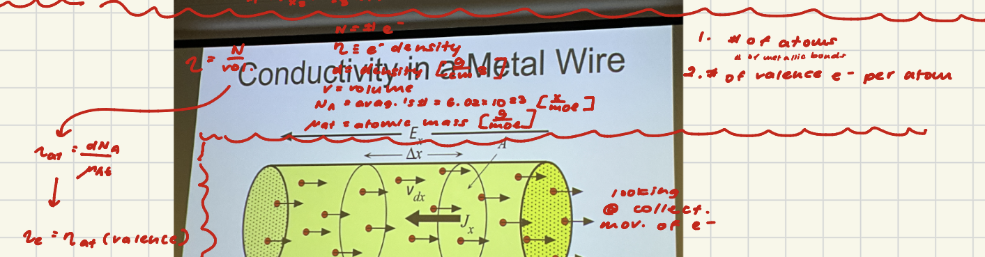
Nav

Nav = 6.022 × 10²3

Homework 1.1:

Multiply moles by Nav to get to calculate number of atoms.

Conductivity Equation

σ = conductivity → how easily electricity flows

e = charge of each electron → 1.6×10^−19 C

n = number of charge carriers per volume → how many things are moving

μ = mobility = ELECTRON drift mobility = charge mobility → how easily/quickly those things can move through the material

Conductivity = how many carriers x how MOBILE they are. n = how many are moving [number of charge carriers PER volume]. mu = HOW EASILY they [the charge carriers] move. Example: Imagine two materials: Material A: Lots of free electrons => high n & Electrons move easily => high mu. [Both lead to] => very high conductivity. More carriers OR more mobility → higher conductivity.

Free electrons

Electrons that are not tightly bound to one specific atoms and can move through a material. Think: In metals: metal atoms have electrons that are relatively loosely attached. These electrons can move throughout the metal, forming a kind of “electron sea.”

Amp

Amp = Coulomb / seconds.

Interatomic Separation

Distance between neighboring atoms.

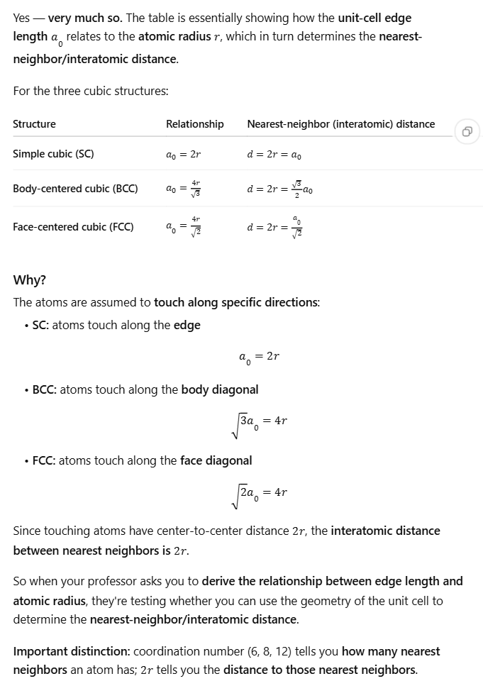
Number of spacings = total distance / distance per spacing.

This is why in problem Homework 1.c, we divided mean free length / interatomic spacing. This gives us how many atomic spacings fit into the electron’s travel distance!

Resistivity Contributions

Resistivity of a material changes with temperature.

alpha_0 => temperature coefficient of resistivity (TCR) at T_0 (temperature of reference.

Resistivity and TCR equations.

eta = empirical fitting factor!!

TCR at a reference temperature equation.