4.2: Least Squares Regression Line

Learning Objectives: 1. Find the least-squares regression line and use the line to make predictions 2. Interpret the slope and the y-intercept of the least-squares regression line 3. Compute the sum of squared residuals

Preview:

regression uses one or more explanatory variables (x) to predict one response variable (y). So, what does this imply of ‘linear’ regression?

The "linear" part is that we will be using a straight line to predict the response variable using the explanatory variable(s)

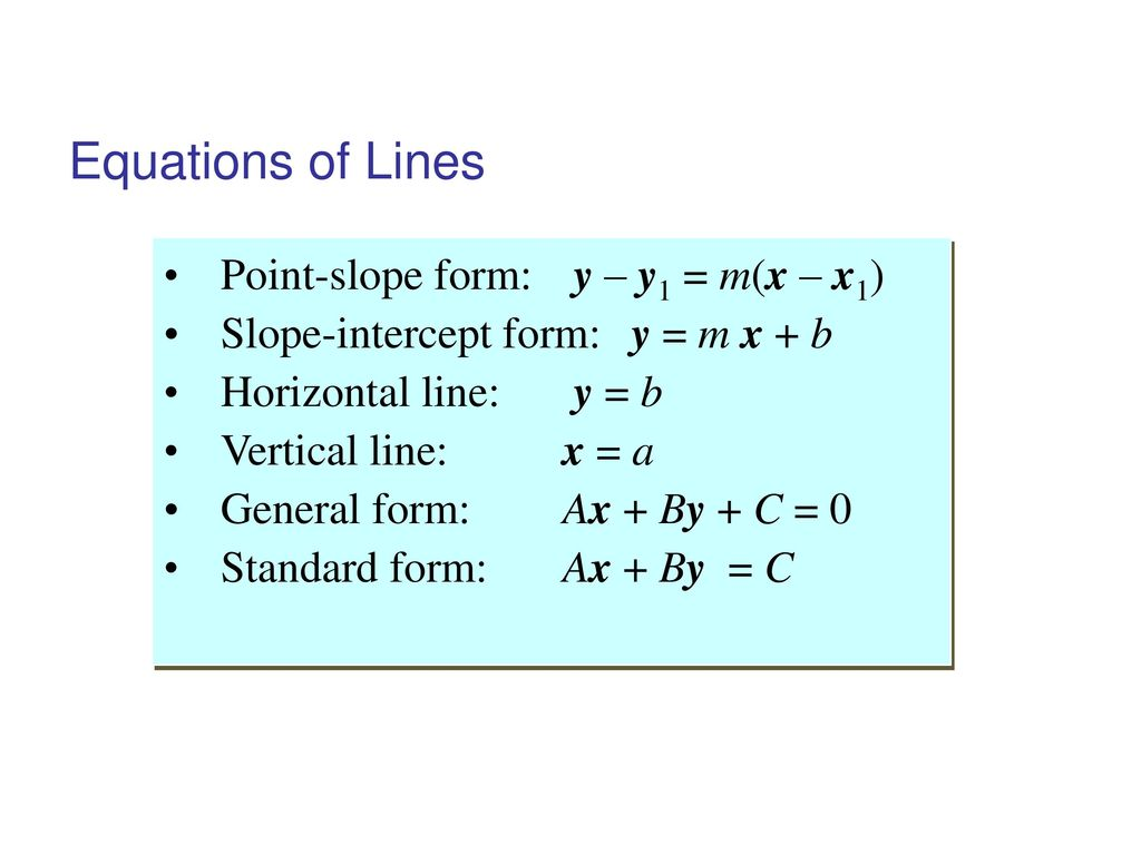
What is the equation for a straight line?

y = mx + b

What is ‘Slope-intercept form’ ?

• Slope-intercept form is a way to write the equation of a straight line

  • • 𝑚 : The slope of the line, which indicates how steep the line is

    • 𝑏 : The y-intercept, which is the point where the line crosses the y-axis

    • 𝑥 : The distance of the line from the x-axis

    • 𝑦 : The distance of the line from the y-axis

What is the y-intercept?

The y-intercept is the location on the y axis where the line passes through;

• the​ y-intercept is found by letting x=0 in an equation and solving for y.

  • When interpreting the​ y-intercept, ask if 0 is a reasonable value for the explanatory​ variable, and if any observations near x=0 exist in the data set. If the answer to either of those questions is​ "no," do not interpret the​ y-intercept.

What is the equation for slope (m) ?

• Slope tells us how steep a line is, like how steep a hill is

  • Rise (y) over Run (x): We find the slope by seeing how much we go up or down (vertical change) for each step to the right (horizontal change).

This version is obviously more complicated than your typical rise/run equation. Thats because we are trying to find the line using two random values of x and y.

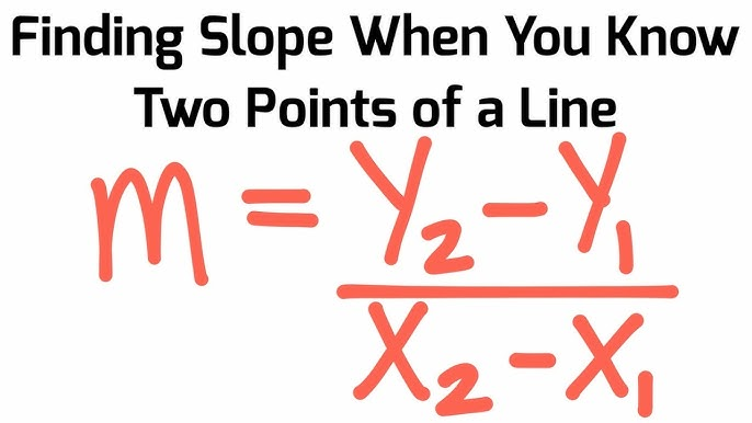
For every one unit increase in x the predicted value of y increases by the value of what?

• the slope

What is the “predicted” y ?

the value of y estimated by the regression line based on the corresponding x value.

• Symbol: Usually represented as "ŷ" (y-hat).

• Calculation: Determined using the regression equation, which takes the form of "ŷ = a + bx" where "a" is the y-intercept and "b" is the slope. 

• Interpretation: For a given x value, the "predicted y" represents the "best guess" for what the corresponding y value would be based on the relationship observed in the data. 

what is the “observed” y

• the actual measured value of the dependent variable (y) in a data set. Essentially, it's the "true" value of y for a given x in your data set.

useful website:

https://online.stat.psu.edu/stat200/book/export/html/244#:~:text=Predicted%20Value%20Symbolized%20as%20(%22y,Sum%20of%20squared%20residuals

What is the ‘Equation of Line’ ?

• Is used to find where a line passes through two points

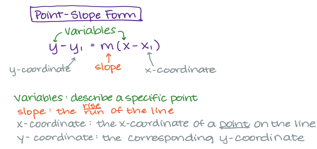
Equations Summary

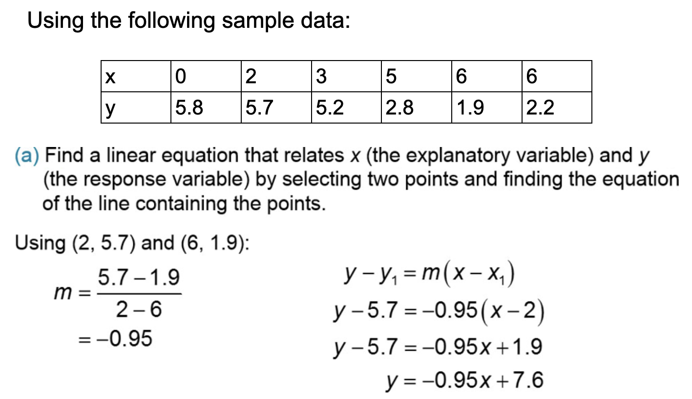
EX: Using Equations to describe Linearly Related Data

What is Residual?

• The difference between the observed value of y and the predicted value of y

  • That is, ‘observed y − predicted y = residual'

    • If it is​ positive, then the observed value is greater than the predicted value.

      • this means that the observed value must be greater than the predicted value.

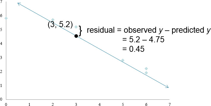
Part 2: Find the residual using the line and the predicted value at x = 3 from the predicted y.

• plug numbers into residual formula

  • = observed y − predicted y

  • = 5.2 − 4.75

  • = 0.45

---

!! NOTICE !! — that we just picked two random points from our data set and based our equation around those two points.

- How do we know we shouldn’t have used two other points?

- How do we know which line would have been the “best line”?

• There is actually a method that ensures we have a line that best fits our data. It uses all of our data points to come up with this line and its equation. Use Minitab to find it, and we should know the method is known as “Least Squares Regression”.

Least Squares Regression Line

response variable is on the y axis and explanatory is on the x axis

Least Squares Regression Line

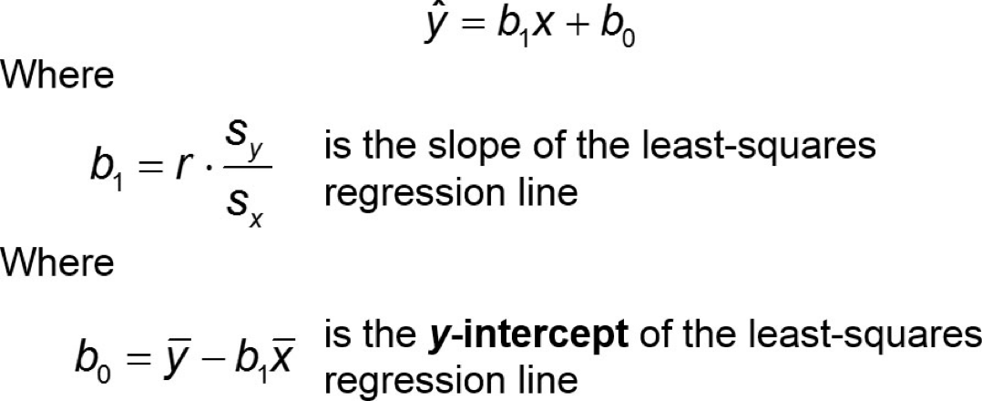
b1 = slope

b0 = y-intercept

EXAMPLE Finding the Least-squares Regression Line

Using the drilling data:

• a) Find the least-squares regression line (round the estimates of slope and intercept to four decimal places)

• b) Predict the drilling time if drilling starts at 130 feet.

• c) Is the observed drilling time at 130 feet above, or below, what we would predict?

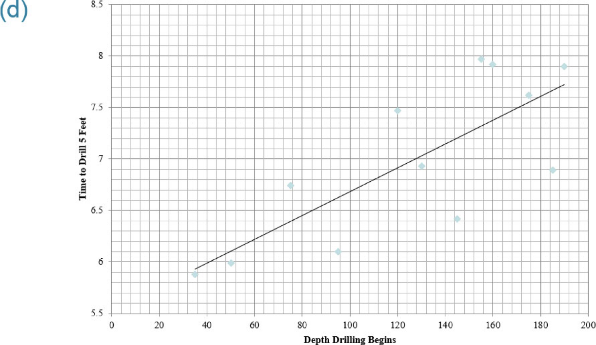
• d) Draw the least-squares regression line on the scatter diagram of the data.

• e) Interpret the slope

• f) Interpret the y-intercept

Depth at Which Drilling Begins, x (in feet)	Time to Drill 5 Feet, y (in minutes)
35	5.88
50	5.99
75	6.74
95	6.1
120	7.47
130	6.93
145	6.42
155	7.97
160	7.92
175	7.62
185	6.89
190	7.9

Use Minitab to get the equation of the regression line

• Stat > Regression > Fitted Line Plot

• Input your variables and click OK.

• The very top is your equation.

If you scroll down, you will see a scatterplot with the regression line overlayed upon it.

---

a) ŷ = 0.0116x + 5.5273

b) ŷ = 0.0116x + 5.5273 —> 0.0116(130) +5.5273 = 7.035

c) The observed drilling time is 6.93 seconds. The predicted drilling time is 7.035 seconds. The drilling time of 6.93 seconds is below what we would predict.

d) **see the picture**

e) The slope of the regression line is 0.0116. For each additional foot of depth we start drilling, the time to drill five feet increases by 0.0116 minutes, on average.

f) The y-intercept of the regression line is 5.5273. To interpret it we must first ask two questions:

1. Is 0 a reasonable value for the explanatory variable? 

2. Do any observations near x = 0 exist in the data set? 

A value of 0 is reasonable for the drilling data (this indicates that drilling begins at the surface of Earth. The smallest observation in the data set is x = 35 feet, which is reasonably close to 0. So, interpretation of the y-intercept is reasonable. 

The time to drill five feet when we begin drilling at the surface of Earth is 5.5273 minutes.

What does it mean when the researcher is using Extrapolation?

• It means they are working outside the scope of the model.

  • When the least-squares regression line is used to make predictions based on values of the explanatory variable that are much larger or much smaller than the observed values

---

Never use a least-squares regression line to make predictions outside the scope of the model !!!!!! (that is, to extrapolate) because we can’t be sure the linear relation continues to exist.