Analysing Quantitative Data

Chapter 10

Data entry and analysis

Main steps involves are:

1. Coding

2. Data entry

3. Tabulation and statistical analysis

Often undertaken by computers but researchers need to develop awareness and understanding of these activities and statistical techniques if to both understand data and present findings in accurate and confident manner.

Coding

Translating responses into numerical form for computer analysis.

Purpose: Allows data to be recognised, stored, and statistically analysed.

Types:

• Pre-coded: Codes already assigned before data collection (closed questions).

• Post-coded: Codes created after collection for open-ended responses.

Steps in Post-coding:

1. List responses → write down all responses.

2. Categorise → group similar answers (e.g. “cheap,” “affordable” = “reasonable price”).

3. Assign numeric codes → input codes into the dataset.

Data Entry

Transferring questionnaire responses to a computer (manually or by optical scanning).

Automated entry: Common in web or computer-assisted surveys.

Data Cleaning:

• Checks for inconsistencies, missing data, or impossible values (e.g. rating 8 on a 1–5 scale).

• Ensures data quality before analysis.

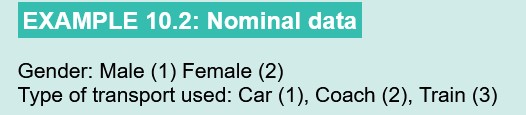
Nominal data scale of measurement

Labels or names; no numerical meaning.

E.g. Gender, Car brand; only frequencies or mode used

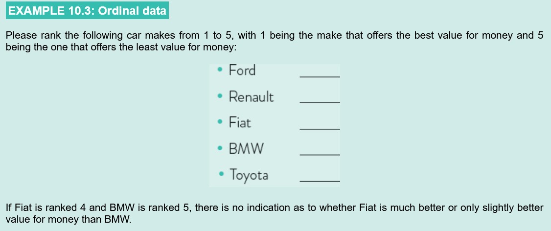
Ordinal data scales of measurement

Indicates order, but not equal intervals.

E.g. Rankings, satisfaction levels

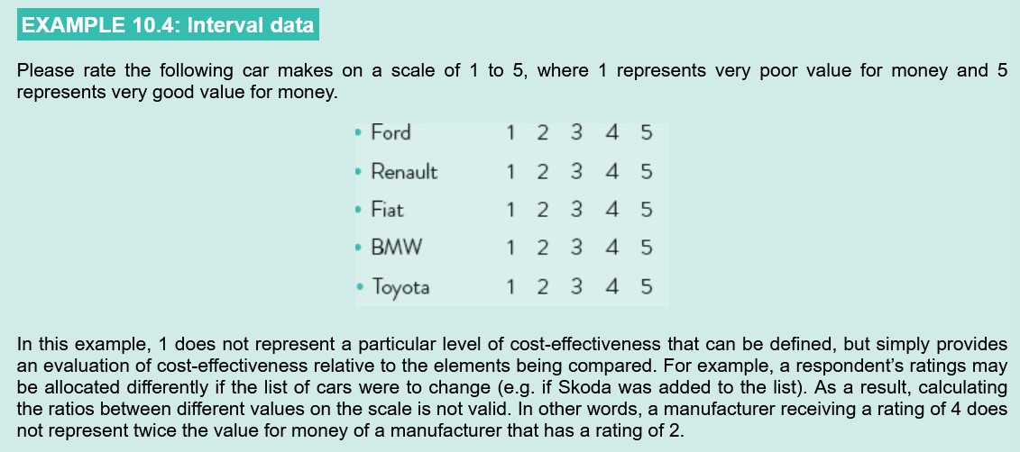
Interval data scale of measurement

Equal intervals; no true zero

E.g. Temperature scale, 1–5 rating; allows mean and SD.

Ratio data scale of measurement 

Equal intervals with true zero.

E.g. Age, income, time; all arithmetic possible.

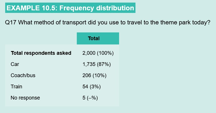
Tabulation and Frequency Distributions

• Tabulation: Summarising data into tables.

• Frequency Distribution: Counts how many respondents chose each option.

• Often shown as numbers and percentages for easy comparison.

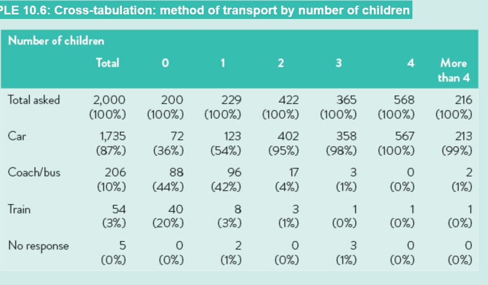
Cross-Tabulations

• Shows the relationship between two or more questions (e.g. “transport type” vs. “number of children”).

• Percentages can be calculated by row, column, or total.

• Helps identify patterns or differences between groups.

Descriptive Statistics

Summarise large data sets with a few key numbers.

Measures of Central Tendency

• Mean: Arithmetic average (interval/ratio data).

• Median: Middle value (less affected by extremes).

• Mode: Most frequent value (any data type).

Measures of Dispersion

Indicates how ‘spread out’ a set of data is. 

• Range: Difference between highest and lowest, calculate the difference between the largest and smallest values in the data e.g. 49 - 39 = 10

• Interquartile Range: Spread of middle 50% of data, calculate by subtracting the first quartile (Q1) from third quartile (Q3) or IQR = Q3 - Q1 

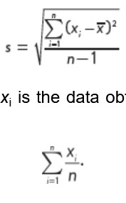
• Standard Deviation (SD): Average distance from the mean. Take square root of sum of squared deviations from mean divided by number of observations -1. Can be compared to see if one set of data is more dispersed than another. 

• n = number of units in sample

• xi = data obtained from each sample unit i

• x- = sample mean value given by E^n i-1 xi/n 

Statistical Significance

• Whether a result is likely due to real difference rather than chance.

• Mathematical difference ≠ Statistical difference.

• Uses significance levels (α), usually 0.05 (5% chance of error).

Hypothesis Testing

• To confirm if sample findings can be generalised to the population.

• Two hypotheses:

  • Null (H₀): No effect or difference.

  • Alternative (H₁): There is an effect or difference.

• Errors:

  • Type I: Rejecting a true null (false positive).

  • Type II: Accepting a false null (false negative).

• α level (significance): Commonly 0.05 → 95% confidence.

Chi-square (X²) statistical test

“Goodness of fit” – difference between observed & expected frequencies

Used in categorial data 

Z test statistical test

Hypothesis about a mean (n > 30).

Used when population variance known

t test statistical test

Used for Hypothesis about a mean (n>30)

Used when population variance is unknown

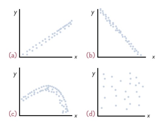
Correlation

Measures strength and direction of relationship between two variables.

• R = +1: Perfect positive.

• R = –1: Perfect negative.

• R = 0: No relationship.

• Pearson’s correlation: For interval/ratio data.

• Spearman’s rank correlation: For ordinal data.

Regression

Describes the relationship mathematically → predicts Y (dependent variable) from X (independent variable).

• Uses least squares method to find best-fitting line.

• R² (Coefficient of Determination): % of variation in Y explained by X.

Multivariate Data Analysis

• Examines two or more variables simultaneously.

• Common techniques:

  • Multiple Regression: Predicts dependent variable using several independents.

  • Discriminant Analysis: Classifies cases into groups (e.g., user vs non-user).

  • Factor / Cluster / Conjoint / Perceptual Mapping: Identify relationships, groupings, and preferences.

Multiple Regression Analysis

• Examines how two or more independent variables affect a single dependent variable.

• Data Requirements:
  Variables should usually be interval or ratio scale (continuous). Nominal variables can sometimes be used if converted into binary (dummy) variables.

• Purpose / Uses in Marketing Research:

  • Estimate how marketing mix elements (e.g. price, promotion) influence sales or market share.

  • Measure how different aspects of customer satisfaction affect overall satisfaction.

  • Predict consumer behaviour (e.g. likelihood to purchase).

• Key takeaway:
  Shows how multiple factors work together to explain or predict outcomes.

Multiple Discriminant Analysis (MDA)

• A technique used to classify individuals into two or more groups (segments) based on their characteristics.

• Example:
  Classifying people as brand users vs. non-users based on income, age, or shopping habits.

• How it Works:

  • Creates a linear combination of independent variables that best separates the groups.

  • Aims to maximize differences between groups and minimize misclassification.

• Use in Marketing Research:

  • Predict which group a new customer might belong to (e.g. likely buyer).

  • Identify which variables are most important in determining group membership.

• Key takeaway:
  Helps researchers segment and classify consumers accurately.

Factor Analysis

• A technique used to simplify data by identifying underlying relationships among variables.
  It reduces many variables into a smaller number of factors (composite variables).

• Example:
  Items like “good value,” “fair price,” and “reasonable cost” might combine into a single “price perception” factor.

• Purposes:

  1. Simplify data – reduce long questionnaires into fewer, meaningful dimensions.

  2. Identify patterns – discover hidden groupings or constructs (like “brand loyalty” or “service quality”).

• Key takeaway:
  Turns large, complex datasets into smaller, easier-to-interpret groups of related variables.

Cluster Analysis

A statistical technique used to classify objects or people into mutually exclusive and exhaustive groups on the basis of tw or more classification variables

Perceptual mapping

An analysis technique that involves the positoning of objects in perceptual space. Frequently used in determining the positioning of brands relative to their competitors.

E.g. Toothpaste manufactuers assessing position of their branded products against competition in terms of protection, price, taste, modernity, freshness of breath, level of whiteness. Respondents asked to evaluate each brand on the attributes.

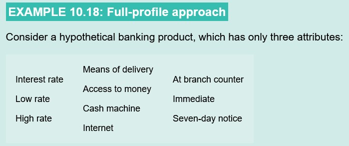
Conjoint analysis

A statistical technique that provides quantitative measure of the relative importance of one attribute over another. Determines what features new product or service should have and how they should be priced.

Respondents pick attributes and pick which ones can be sacrificed, find a form of compromise solution.

Trade-off data collected by:

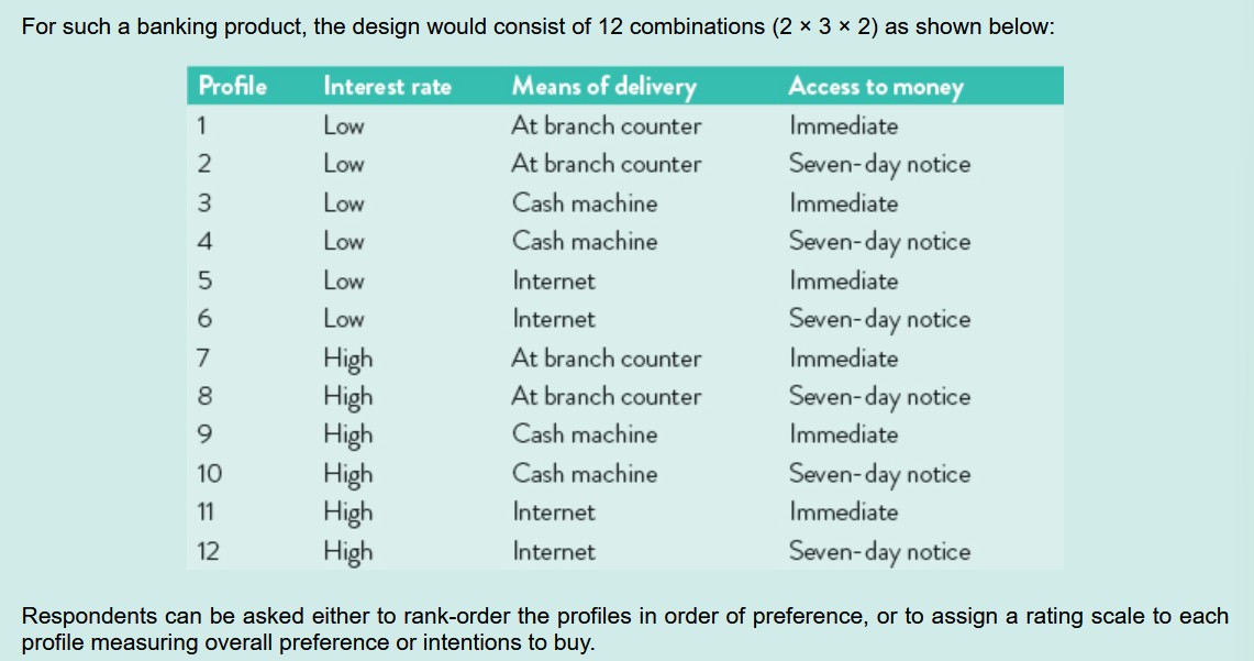
Respondents either asked to consider 2 attributes at a time or to assess full profile of attributes at once.

Full-profile considers all attributes when buying a product but number of sttributes increasing means task of judging individual profiles is complex and hard to take account of all variations in attributes.

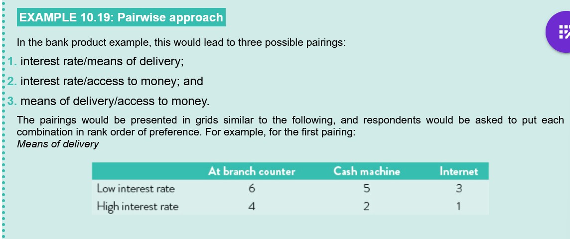
Pairwise (trade-off approach) conjoint analysis

Attributes are presented in pairs instead

Lacks realism of full-profile approach but easier for respondent to make judgements between 2 attributes. Ensure not too many attributes as task can be repettive and boring. 

If many attributes, 2-stage approach may be adopted where respondents classify attributes in various groups relating to imporatance. Pairings set up with least important attributes. 

Can allow respondents to input decisions directly to specialist computer package, computer decides based on previous responses the next attributes to access, not showing those they rejected. 

Enables researcher to make estimates of potential market share for each of the potential designs of products or services.

However, may not totally reflect reality as consumer unlikely approach purchasing decisions with rational and deliberate manner, may not be fully aware of product features when buying or influenced by branding/ads.