Methods: Chapter 18-21 - Calculus

Smash that calculus!

Average Rate of Change

• Measures how much a function changes on average over an interval

• Formula: (f(b) - f(a)) / (b - a)

• It's the gradient of the secant line through (a, f(a)) and (b, f(b))

• For motion, it's average speed = distance ÷ time

The Derivative

Key Concepts

• A secant is a line through two points on a curve.

• A tangent is a line that touches the curve at one point with the same gradient.

• The instantaneous rate of change is the gradient of the tangent.

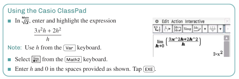
First Principles Definition

• Derivative: Slope
  f'(x) = lim (h → 0) [(f(x + h) - f(x)) / h]

Approximating Derivatives

• For small h:
  f'(a) ≈ (f(a + h) - f(a)) / h

Tangents

• Gradient of tangent at x = a:
  👉 f'(a)
  So at point (1, −2), if f'(1) = −3, the tangent’s slope = -3.

Notes

• Derivative exists only if the limit exists.

• All polynomials are differentiable.

Derivative Rule - Basic

Power Rule
If f(x) = xⁿ, then
👉 f'(x) = n xⁿ⁻¹
(Proven using the binomial theorem.)

Special Cases

• Constant:
  f(x) = c ⇒ f'(x) = 0

• Linear:
  f(x) = mx + c ⇒ f'(x) = m

Add-Ons

• Multiply:
  f(x) = k ⋅ g(x) ⇒ f'(x) = k ⋅ g'(x)

• Sum:
  f = g + h ⇒ f' = g' + h'

• Difference:
  f = g − h ⇒ f' = g' − h'

🧪 Examples
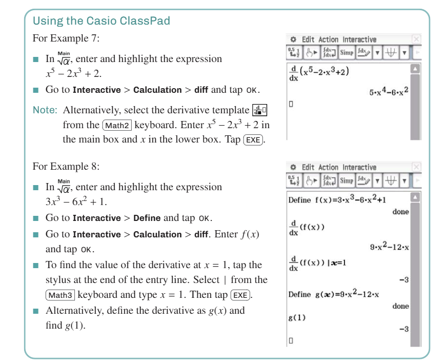
f(x) = x⁵ − 2x³ + 2
👉 f'(x) = 5x⁴ − 6x²

f(x) = 3x³ − 6x² + 1
👉 f'(x) = 9x² − 12x, so f'(1) = −3

Lebiniz Notation

If y = x³, write:
👉 dy/dx = 3x²
(Same idea, different style. Don't treat dy/dx like a fraction.)

Differentiating xⁿ where n is a negative integer

• Power rule still applies: derivative of xⁿ is nx^n-1

• Domain: x ≠ 0 (no zero allowed because of division)

• Examples:
   • d/dx (1/x) = -1/x²
   • d/dx (x⁻³) = -3x⁻⁴

• Constants → derivative is 0

• Tangent slope = derivative evaluated at point

• Negative powers = fractional forms, watch domain carefully!

Differentiating rational powers (x to the p over q)

• Use first principles for simple powers like x¹ᐟ², x¹ᐟ³

• Key identity: aⁿ - bⁿ = (a - b)(aⁿ⁻¹ + aⁿ⁻²b + … + bⁿ⁻¹)

• Use chain rule for general rational powers:
   • If y = xᵖ⁄q, write y = (x¹⁄q)ᵖ
   • Then dy/dx = (p/q) × x^(p/q - 1)

• Domain: x > 0 (to avoid issues with roots of negatives)

• Applies to any real non-zero power: derivative of xᵃ is a × xᵃ⁻¹

• Examples:
   • d/dx (x²ᐟ³) = (2/3) × x⁻¹ᐟ³
   • d/dx (4x²ᐟ³) = 4 × (2/3) × x⁻¹ᐟ³

• Graphs of fractional powers are smooth for x > 0 but tricky near 0 for some powers

Chain Rule

• The chain rule is like mom(son) — a function inside a function.

• To differentiate y = mom(son), do: derivative = son' × mom'(son).

Break y = f(g(x)) into:

• Son = g(x) (inner function)

• Mom = f(u) (outer function, with u = son)

Steps:

1. Differentiate inner: son' = g'(x)

2. Differentiate outer at son: mom'(son) = f'(u) at u = g(x)

3. Multiply: dy/dx = mom'(son) × son'

Example: y = (3x + 4)^20

• son = 3x + 4, son' = 3

• mom = u^20, mom' = 20u^19

• derivative = 20(3x + 4)^19 × 3 = 60(3x + 4)^19

Official formulas:

Chain rule (function notation):
(f ∘ g)'(x) = f'(g(x)) × g'(x)
where (f ∘ g)(x) = f(g(x))

Chain rule (Leibniz notation):
dy/dx = dy/du × du/dx

Tangents & Normal

• Derivative gives the gradient of the tangent at any point on a curve.

• Tangent line equation at (x₁, y₁):
  y − y₁ = f'(x₁)(x − x₁)

• Normal line is perpendicular to the tangent.

• If tangent gradient = m, normal gradient = −1/m

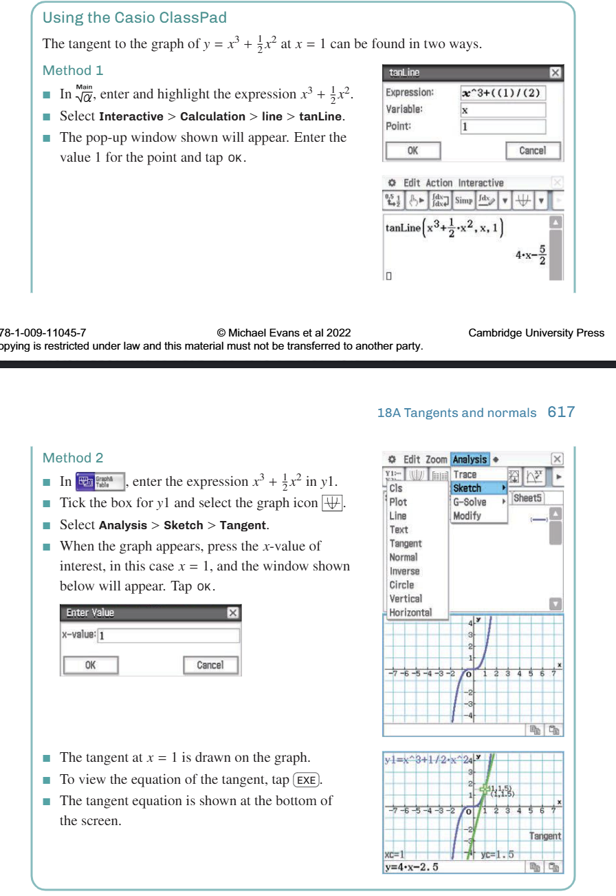
Example tangent:
For y = x³ + ½x² at x = 1:

• Point: (1, 3/2)

• Gradient: f'(1) = 4

• Tangent: y − 3/2 = 4(x − 1) → y = 4x − 5/2

Example normal:
For y = x³ − 2x² at (1, −1):

• Tangent gradient: f'(1) = −1

• Normal gradient: 1

• Normal: y + 1 = 1(x − 1) → y = x − 2

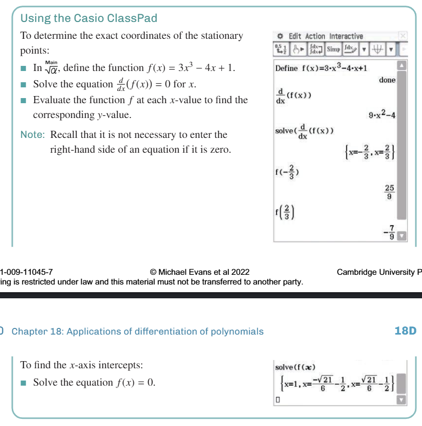
Stationary Points

• A point (a, f(a)) on curve y = f(x) is stationary if the derivative = 0 at x = a.

• In symbols: f'(a) = 0 or dy/dx = 0 at x = a.

• At stationary points, the tangent is horizontal (parallel to x-axis).

Types:

• Local Maximum: f′(x) changes from + to – (peak)

• Local Minimum: f′(x) changes from – to + (valley)

• Inflection Point: f′(x)=0, no sign change (flat but no turn)

Turning Points: Local max and min only.

Examples:

1. y = 9 + 12x − 2x²

   • dy/dx = 12 − 4x

   • Set to 0: 12 − 4x = 0 → x = 3

   • Stationary point: (3, 27)

Steps to solve max/min problems

• Draw & label diagram; define variables and limits.

• Express quantity to max/min as a single-variable function.

• Find stationary points where derivative = 0.

• Test points to identify local max/min/neither.

• Check function values at domain endpoints if any.

Second Derivative

The derivative of the first derivative:
f″(x) = d/dx (f′(x))

Example:
If f(x) = 2x² + 4x + 1, then f′(x) = 4x + 4 and f″(x) = 4

In physics:
position = x(t), velocity = dx/dt, acceleration = d²x/dt²

Example:
f(x) = 3x³ + 2x⁻¹ + 1
f′(x) = 9x² − 2x⁻²
f″(x) = 18x + 4x⁻³

Second Derivative Test

If f ''(x) > 0, the function is concave up ⇒ local minimum
If f ''(x) < 0, the function is concave down ⇒ local maximum
If f ''(x) = 0, the test is inconclusive

Use it at critical points where f '(x) = 0

Sketching Graphs

Steps for sketching graphs:

• Find x-axis and y-axis intercepts and stationary points.

• Identify where the graph is increasing and decreasing.

• Determine the nature of each stationary point:
  • local maximum
  • local minimum
  • stationary point of inflection

• Identify vertical asymptotes.

• Understand the behavior as x → +∞ and x → −∞.

Graphs of the derivative function

• Sign of derivative tells slope direction of original graph:

  • If f′(x) > 0, graph slopes up (increasing).

  • If f′(x) < 0, graph slopes down (decreasing).

  • If f′(x) = 0, potential stationary point.

• Intervals:

  • Increasing where f′(x) > 0.

  • Decreasing where f′(x) < 0.

  • Stationary points where f′(x) = 0.

• Derivative tests:

  • f′(x) > 0 → function strictly increasing on interval.

  • f′(x) < 0 → function strictly decreasing on interval.

  • But watch out: strictly increasing doesn’t always mean f′(x) > 0 everywhere (like f(x) = x³).

• Gradient & angle connection:

  • Gradient m = tan(θ), where θ is angle with x-axis.

  • E.g., θ=45° means m=1; θ=135° means m=−1.

• Use derivative to find tangents at given slopes or angles.

CAS: Plot graph of normal function and derivative function.

Families of Functions and Transformations

Given f(x) = (x − a)²(x − b), with a, b positive and b > a:

a) Derivative: f'(x) = (x − a)(3x − a − 2b) (found using CAS)
b) Stationary points: (a, 0) and ( (a + 2b)/3 , value from f(x) )
c) Local max at (a, 0) because f'(x) changes from positive to negative around a
d) Given stationary points at x=3 and x=4, then:

• a = 3

• (a + 2b)/3 = 4 → b = 9/2

Limits and Continuity

Limit Definition
Limit (lim): As x approaches a, f(x) gets arbitrarily close to L. Written as lim x→a f(x) = L.

For many functions (especially polynomials), lim x→a f(x) = f(a).

If f is not defined at a, factor or simplify to find the limit.

Algebra of Limits (if limits exist):
lim x→a (f(x) + g(x)) = lim x→a f(x) + lim x→a g(x)
lim x→a (k f(x)) = k lim x→a f(x)
lim x→a (f(x) g(x)) = lim x→a f(x) × lim x→a g(x)
lim x→a (f(x) / g(x)) = (lim x→a f(x)) / (lim x→a g(x)), if lim x→a g(x) ≠ 0.

Left and Right Limits:
lim x→a⁻ f(x) is the limit approaching from the left.
lim x→a⁺ f(x) is the limit approaching from the right.

Limit exists only if both are equal.

Continuity at x = a:
f is continuous at a if:

• f(a) is defined, and

• lim x→a f(x) = f(a).

Otherwise, f is discontinuous at a.

Note:
Polynomials are continuous everywhere.

When is a function differentiable?

When is a function differentiable?

• A function f is differentiable at x = a if the limit of [f(a+h) - f(a)] / h as h → 0 exists.

• Polynomials are differentiable everywhere (for all real numbers).

Example: Modulus function

• f(x) = x if x ≥ 0; f(x) = -x if x < 0

• Gradient of secant between (0,0) and (h, f(h)) is:

  • 1 if h > 0

  • -1 if h < 0

• Left and right limits do not match → derivative does not exist at 0

• So, f is not differentiable at x = 0.

Derivative function for modulus

• f'(x) = 1 if x > 0

• f'(x) = -1 if x < 0

---

Piecewise differentiability and smooth joins

• Some piecewise functions are differentiable everywhere if their joins are smooth.

Example 1

• f(x) = x² + 2x + 1 if x ≥ 0; f(x) = 2x + 1 if x < 0

• Derivative: f'(x) = 2x + 2 if x ≥ 0; f'(x) = 2 if x < 0

• f'(0) exists and equals 2 → smooth join → differentiable at 0

Example 2

• f(x) = x² + 2x + 1 if x ≥ 0; f(x) = x + 1 if x < 0

• Derivative: f'(x) = 2x + 2 if x > 0; f'(x) = 1 if x < 0

• f'(0) does not exist (left and right limits differ)

• Differentiable everywhere except at 0

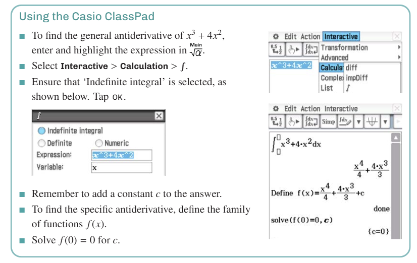
Antidifferentiation of Polynomials

• Antidifferentiation: Finding a function from its derivative.

• Functions with the same derivative differ by a constant (vertical shifts).

Rules:

• If F'(x) = f(x), then ∫f(x) dx = F(x) + c (differentiation lose components; any constant).

• Reverse power rule: ∫xⁿ dx = xⁿ⁺¹ / (n + 1) + c, for n ≠ -1.

• Linearity:

  • ∫[f(x) + g(x)] dx = ∫f(x) dx + ∫g(x) dx

  • ∫[f(x) − g(x)] dx = ∫f(x) dx − ∫g(x) dx

  • ∫k f(x) dx = k ∫f(x) dx (k constant)

Finding specific antiderivatives (with initial conditions):

• Use general ∫f'(x) dx + c

• Plug known point to solve for c

• Example: f'(x) = 5x, f(0) = 6 → f(x) = 5x²/2 + 6

Examples:

• ∫3x⁵ dx = 3 × (x⁶ / 6) + c = (1/2) x⁶ + c

• ∫(3x² + 4x³ + 3) dx = x³ + x⁴ + 3x + c

• Find f(x) if f'(x) = x³ + 4x² and f(0) = 0:

  • ∫(x³ + 4x²) dx = x⁴/4 + 4x³/3 + c

  • Use initial condition f(0) = 0 → c = 0

  • So f(x) = x⁴/4 + 4x³/3

Antidifferentiating rational powers

• ∫ x^r dx = x^(r+1) / (r + 1) + c

• r must be a rational number, not -1

• Domain of x depends on the value of r

• ∫ (2x^-4 + 6x) dx = -2/3 x^-3 + 3x² + c

Finding the Exact Area: The Definite Integral

• It gives the exact area under a curve:
  ∫ₐᵇ f(x) dx = [F(x)] a b = F(b) − F(a)

• F is any antiderivative of f (thanks to the Fundamental Theorem of Calculus)

• It’s the limit of Riemann sums as n → ∞

• Works when f is continuous on [a, b]

• This is called the definite integral of f(x) with respect to x from x = a to x = b.

• This is called the fundamental theorem of calculus (cool!).

Extended, complex version of definite integral

• The definite integral ∫ₐᵇ f(x) dx is the limit of a sum:
  ∫ₐᵇ f(x) dx = limₙ→∞ Σᵢ₌₁ⁿ f(xᵢ*)Δx

• Δx = (b − a)/n

• xᵢ* is a sample point in the i-th subinterval

• This sum approximates area under f(x); the limit gives the exact value

Signed area vs Total area

• Signed area = ∫ₐᵇ f(x) dx → positive above x-axis, negative below
• Total area = ∫ₐᵇ |f(x)| dx → all areas positive

• If f(x) ≥ 0 on [a, b]: Area = ∫ₐᵇ f(x) dx
• If f(x) ≤ 0 on [a, b]: Area = −∫ₐᵇ f(x) dx

• If f(x) changes sign at x = c (a < c < b):
 → Area = −∫ₐᶜ f(x) dx + ∫꜀ᵇ f(x) dx
 → Or Total area = ∫ₐᵇ |f(x)| dx

• Geometry tricks:
 – Triangle: ½ × base × height
 – Trapezium: ½ × (a + b) × height

Properties:

• ∫ₐᵇ f(x) dx = −∫ᵦₐ f(x) dx
• ∫ₐᵃ f(x) dx = 0
• ∫ₐᵇ [k·f(x)] dx = k·∫ₐᵇ f(x) dx
• ∫ₐᵇ [f(x) ± g(x)] dx = ∫ₐᵇ f(x) dx ± ∫ₐᵇ g(x) dx
• ∫ₐᵇ f(x) dx = ∫ₐᶜ f(x) dx + ∫꜀ᵇ f(x) dx

Tips:

🧠 Use the split rule when the function changes sign or form mid-way.

Estimating Area

Divide the interval [a, b] on the x-axis into n equal subintervals [x₀, x₁], [x₁, x₂], [x₂, x₃], …, [xₙ₋₁, xₙ] as illustrated.
Estimates for the area under the graph of y = f(x) between x = a and x = b:

Left-endpoint estimate
Lₙ = (b − a)/n × [f(x₀) + f(x₁) + ··· + f(xₙ₋₁)]

Right-endpoint estimate
Rₙ = (b − a)/n × [f(x₁) + f(x₂) + ··· + f(xₙ)]

Trapezoidal estimate
Tₙ = (b − a)/(2n) × [f(x₀) + 2f(x₁) + 2f(x₂) + ··· + 2f(xₙ₋₁) + f(xₙ)]
These methods work for any continuous function on [a, b], regardless of whether the graph is increasing or decreasing.