PSYC2001 Final

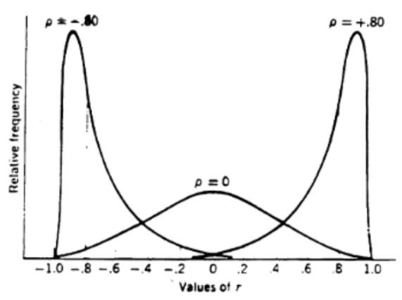
Shape of sampling distribution of correlation

Not normal (symmetric or bell-shaped).

Shape depends on true correlation and sample size.

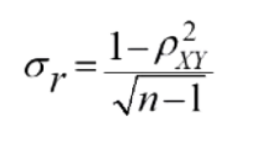
Standard deviation of correlation

• Indicates how much the sample correlation r varies across samples.

• Depends on true correlation pxy and sample size n.

  • Larger n → smaller standard deviation.

    • Less variability = more precise estimate.

  • Larger pxy → smaller standard deviation.

    • When pxy is near +_1 = sampling distribution is more concentrated.

    • Sample correlations tend to be closer to true value.

Interpreting intercept in regression equation

Tells you the predicted value of Y when X = 0.

E.g. Y’ = 48 + 3.2X

Intercept = 48

When study hours = 0, the predicted exam score is 48.

Represents the starting point of the regression line.

Interpreting slope of regression equation

Tells you predicted outcome changes for every 1-unit increase in the predictor variable (X).

E.g. Y’ = 48 + 3.2X

Slope = 3.2

For every hour studied, the predicted exam score increases by 3.2 marks.

Slope describes the direction and rate of change.

Direction and rate of change based on slope in regression equation

Positive slope (+b) = as X increases, Y increases

Negative slope (-b) = as X increases, Y decreases

Larger slope = stronger rate of change.

Empirical rule of standardised residual

68% of the data falls within 1 standard deviation of the mean.

95% of the data falls within 2 standard deviations of the mean.

99.7% of the data falls within 3 standard deviations of the mean.

Size of prediction error

Absolute value (ignore + or -) tells you whether the error size is small or large.

0 - 1: small error

• Actual score is close to predicted score

1 - 2: moderate error

• Prediction is somewhat inaccurate but still reasonable.

2 - 3: large/unusual error

• Model predicted poorly in this caseZ

Beyond 3: very large prediction error.

• Observation may not fit regression model.

Mean of sampling distribution of rxy

The mean is pxy

The expected average value of the sampling distribution of rxy is the true population correlation pxy.

Prediction (foundational)

• Using scores on one variable (X) → predict another variable (Y).

  • X = independent or predictor variable.

  • Y = dependent or criterion variable.

• Based on known correlation between them rxy (both X and Y info are avail).

• Use regression/prediction equation.

Single and multiple regression in prediction

Single regression: one X and one Y.

Multiple regression: more than one X.

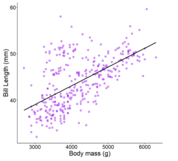
• E.g. Y = bill length.

• X1 = body mass.

• X2 = species.

• X3 = flipper length.

Regression equation

In simple regression, the equation describes a straight line that best fits the data in 2-dimensional (X-Y) space.

Prediction with z-scores

Amount by which prediction differs from 0 depends on the strength of r.

If r = +1.0

• Predict Zy’ = Zx.

If r = 0.0

• Predict Zy’ = 0.

If r is between 0 or 1.

• Provides some information to help us predict Y.

• But the relationship is not perfect (confounding factors/noise).

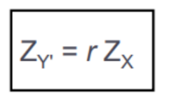
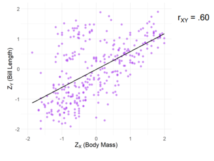
Z-Score Prediction

• Gives prediction for Y based on X but depends on the size of r.

• This equation describes line of best fit through the scatter plot of Zy against Zx.

• This regression line passes through origin (0,0) and has a slope of r.

R vs R²

R (Pearson correlation coefficient)

• Measures strength and direction of a linear relationship between two variables.

• Range: -1 to 1.

• Indicates: positive, negative, how closely points fit a line.

• E.g. R = -0.9 → variables have a strong negative relationship.

R² (Coefficient of determination)

• Represents the proportion of variance in the dependent variable explained by the model.

• Range: 0% to 100% (always positive).

• Says what percentage of the variation in Y is explained by X.

• E.g. R² = (-0.9)² = 0.81 → the model explains 81% of the variance.

?

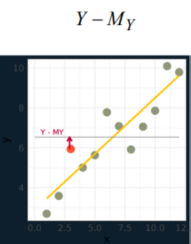
Deviation

• The difference between an observed value (Y) and its mean (My).

• How far an actual data point is from the average.

?

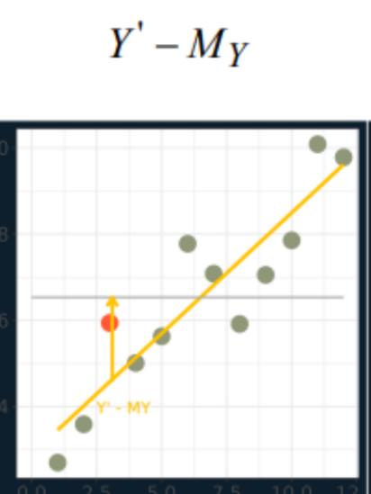
Prediction

• The estimated value from the regression model.

?

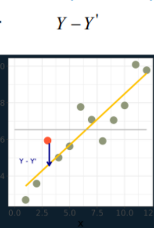
Error (residual)

• The difference between the observed value and the predicted value.

  • How far is the prediction Y from the data point.

• This is the part of the deviation that the model could not explain.

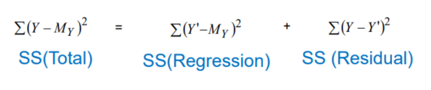
Total variability

Equation explains that total variability (sum of squares) can be split into the explained part (regression) and unexplained part (residual).

SS (Regression): How well the model predicts Y using X.

SS (Residual): The variability not explained by the model (noise).

Line of best fit and error

• Regression line is considered line of best fit because it minimises overall prediction error.

• Defined so that SS (residual) / noise is minimised → least squares criterion.

• Makes it the most accurate linear model for predicting Y from X.

When r is large

• Y values tend to cluster more closely around the predicted Y’ values.

• Larger proportion of the variance in Y is explained by the prediction.

When r is small

• Y values are more spread out around Y’.

• Less of the variance is explained.

• Leads to larger prediction errors.

Assumptions for linear regression

1. In the population, X and Y form a bivariate normal distribution.

2. Linearity: X and Y are linearly related.

• I.e. means of distributions of Y score for each X fall on a straight line.

3. Homoscedasticity: variance of distributions of Y scores for each X score is the same.

When assumptions for linear regression are met

• Can use prediction equation to estimate:

  • The percentage of cases that are a certain distance from their predicted value.

  • The probability of a score being a certain distance from its predicted value.

• Standard error of the estimate (Syx)

  • Measures predictive error.

Standard error of estimate (Syx)

• Measures the average amount of error when predicting Y from X using the regression line.

• Tells us how far predicted values Y’ are from the actual observed values Y on average.

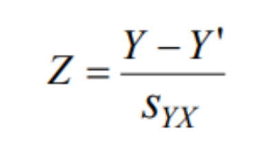
Standardised residual

Finds how unusual it is to obtain a particular Y, given Y’.

Also using table of areas under the normal curve to obtain likelihood statements.

E.g. Syx = 4.394 → for any X, about 68% of actual Y scores will be within 4.394 (one standard deviation) of Y’.

Factorial design language

2 × 3 → Two factors with three levels.

Example:

Factor A: Fertiliser amount (low - 10g, medium - 20g, high - 30g).

Factor B: Watering frequency (low - monthly, medium - weekly, high - daily).

3 × 2 × 2 → Three factors, one with 3 levels, the other two with 2 levels.

Example - all IVs:

Work environment (3 levels): quiet, open-plan, remote.

Music background (2 levels): music or no music.

Task type (2 levels): creative task or analytic task.

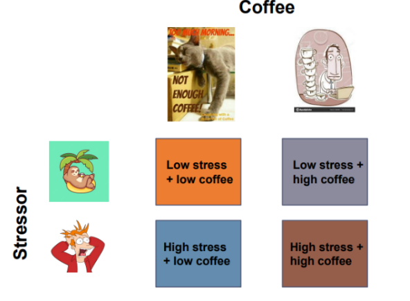
Proper factorial language for this example

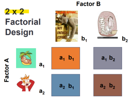
Main effect of factorial design

Effect of a factor, averaged over levels of other factors.

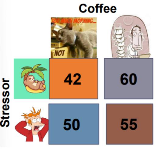
E.g. the effect of stressor, averaged over coffee levels.

2 factors = 2 main effects.

E.g. main effect of stressor

(42 + 60)/2 = 51

(50 + 55)/2 = 52.5

= 1.5 points

Marginal mean

The averages for one factor, calculated by averaging across all levels of other factors (usually corner).

Main effects vs interactions in factorial designs

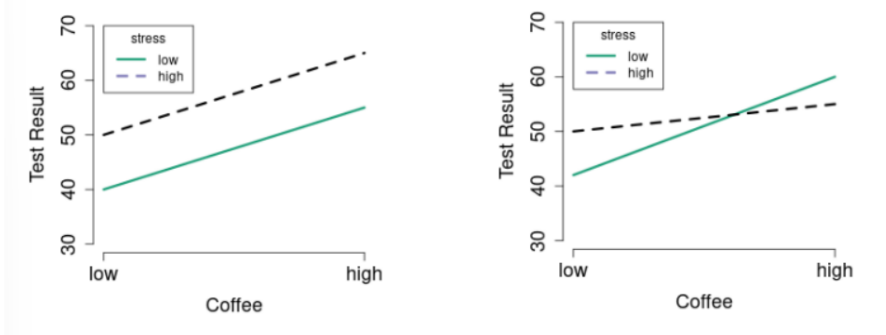
Interactions: slopes are not parallel.

• Parallel = two MEs do not interact (or depend on each other for their values).

• Therefore, it would be concluded that the effects of two variables are independent of each other.

Mixed 2 × 2 design

One factor is within and one is between.

There would be 2 groups and each participant would be tested twice.

Interactions in factorial designs

Arises when the effect of one factor differs over levels of the other factor.

• Quantified by calculating ‘difference of differences’.

E.g. effect of Length for action movies (A)

Short action mean - long action mean

E.g. effect of Length for drama movies (B)

Short drama mean - long drama mean

A - B = interaction

Why does the sample variance tend to underestimate the population variance?

• Sample mean is closer to the sample data points than the true population mean.

• Results in smaller squared deviations.

• Sample data is used to calculate its own mean → it is less ‘spread out’.

  • Leading to an artificially low variance estimate.

Line of best fit

• Also known as a regression line.

• Passes through the origin (e.g. does not pass through y = 1).

• Exists in a 2-dimensional space.

• Can be described with Zy’ = rZx.

Prediction variables (Y and X)

• Y: dependent or criterion variable.

• X: independent or predictor variable.

What is NOT an important element of multiple factorial design?

• Two or more dependent variables.

Whilst it is possible to have multiple dependent variables, it is not as important as:

• Two or more independent variables.

• The belief that no one factor will exert its effect independently.

• The possibility of the interaction of main effects.

When performing a correlation power analysis, what does gamma y refer to?

The magnitude of the population correlation to be detected.

What percentage is power typically aimed at and why?

80%

• To avoid false negatives/Type II errors.

What can be manipulated to produce higher power?

Increasing sample size.

• Less variance → more precise estimates → greater statistical power.

• Higher variability reduces statistical power to detect true difference.

What values are fixed when calculating statistical power?

Gamma

Standard deviation

Alpha 2-tailed

Relationship between power and confidence intervals

Closely related.

• Higher power (lower type II error) results in narrower, more precise confidence intervals for a given effect size.

• Width of confidence interval is a direct measure of how precise the estimated effect is.

• Both influenced by sample size (larger N → more narrow CI → more precise estimates).

• Decreasing the false-positive rate (i.e. a = 99% instead of 95%) → increases width of Ci and decreases statistical power.

How power provides a distinction between statistical and practical significance

• Specifies a minimum effect of interest.

• Any effect smaller than that value is of no practical importance (even if null hypothesis is technically false).

• Focus should be on whether null hypothesis is false to an important degree.

Factors affecting power

1. Size of alpha

• Decreases → moves cutoff to right (less power).

• Range where null hypothesis is tested increases (Zc) → more Type II errors → less power.

2. Directionality (2-tailed)

3. Effect size (gamma)

• Bigger the effect → easier to detect (more power).

4. Size of standard deviation.

• Affect standard error (where lower is better).

• Increases → increases standard error → less power.

5. Number of participants.

• Increases → decreases standard error → more power.

Cohen guideliens

Small effect size y = .2

Medium effect size y = .5

Large effect size y = .8

Gamma and delta units

Gamma:

Calculates difference, in units of standard deviation.

Delta:

Calculates difference, in units of standard error (used for power).

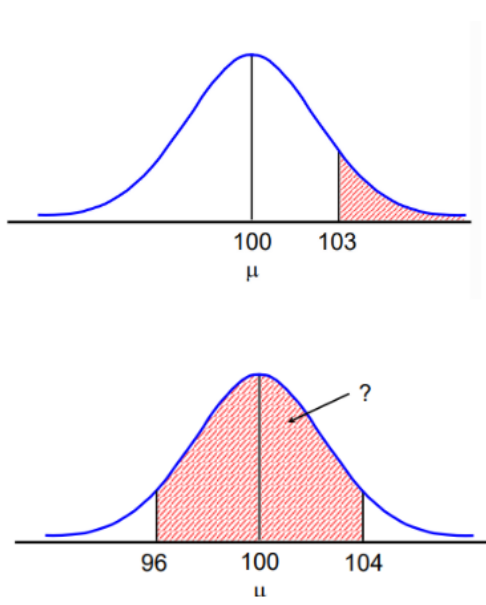
Z-Scores: Chance of getting a score (steps)

1. Calculate standard error.

2. Calculate Z-score using formula.

3. Find area on table.

One side: 0.5 - area = answer.

Two sides: area x 2.

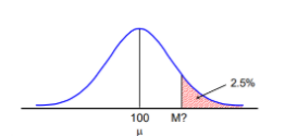
Z-Score: What value will be exceeded by __% of the sample means? (Steps)

1. Calculate standard error.

2. 0.5 - area = __

3. Find z-score that corresponds to area.

4. Convert Z to M by rearranging formula.

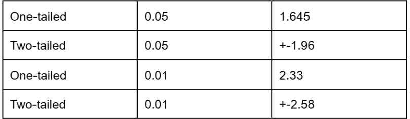
Critical Z values

Type I error

False positive.

• When the null hypothesis is true but is wrongly rejected.

• Concluding a significant effect/difference exists, when it does not.

Type II error

False negative.

• When the null hypothesis is false but was not rejected (miss).

• An effect/difference does exist but was not detected by the study.

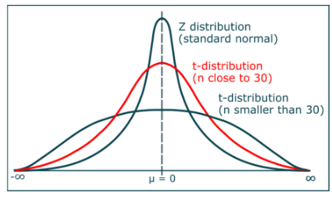
T-Distribution Properties

• Shape changes depending on df.

  • Larger df → normal curve.

  • Small df → wide curve, flatter peak.

• Df >_ 1 = mean of t-distribution always 0.

• More normal → less uncertainty.

  • Bigger samples: t and z almost identical.

Assumptions for independent means.

1. Normal distribution.

2. Population variances are equal.

3. Observations are independent.

All true → test is reliable.

Not met → may effect error rate.

Robustness

• How reliable an independent samples t-test is when not all conditions are met.

• Test makes as much Type I errors as expected (close to alpha level).

• Assumptions.

  • Violation against normality → still robust.

  • Violation against variance → still robust.

  • Violation against independence → not robust.

Violation of equal variance.

When n1 =/= n2, it depends on which group has the larger variance.

T-test is either conservative or liberal.

Conservative t-test

Larger sample = larger variance → conservative.

• Actual Type I error rate is less than alpha rate.

• Slight overestimation = more robust.

• Produces a larger standard error → smaller t-value → harder to reject null hypothesis.

  • Reduces risk of Type I error.

Liberal t-test

Larger sample = smaller variance → liberal.

• Actual Type I error rate is more than alpha rate.

• Underestimates variability = less robust.

• Produces a smaller standard error → larger t-value → easier to reject null hypothesis.

  • Higher risk of Type I error.